Package version
Overview
Teaching: 5 min
Exercises: 5 minQuestions
How do you know your installed package versions?
How do you instal a certain version of a package?
Objectives
Install the package versions used for this tutorial
Scientific reproducibility is key for the advancement of Science. In this first episode, we will check that you have the same package versions that we will use throughout the tutorial.
We will use the function packageVersion from the utils package to register the package version we are using for this tutorial.
It only takes a single element character vector as input, so you will have to type the function and the package name each time, as follows:
packageVersion("rotl")
packageVersion("ape")
packageVersion("devtools")
packageVersion("stringi")
packageVersion("datelife")
packageVersion("datelifeplot")
[1] '3.0.11'
[1] '5.5'
[1] '2.4.2'
[1] '1.7.4'
[1] '0.3.2'
[1] '0.1.0'
Alternatively, you can create a character vector of package names and use an lapply to get versions of all packages at once:
packages <- c("rotl", "ape", "devtools", "stringr", "datelife", "datelifeplot")
names(packages) <- packages

lapply(packages, packageVersion)
$rotl
[1] '3.0.11'

$ape
[1] '5.5'

$devtools
[1] '2.4.2'

$stringr
[1] '1.4.0'

$datelife
[1] '0.3.2'

$datelifeplot
[1] '0.1.0'
If you have older versions of the packages, you can update them with install.packages, as if you were to install them anew, following instructions in the setup of this tutorial.
The function update.packages does not allow updating single packages. Instead, it will try to update all packages already installed.
You can use it as follows:
update.packages(ask = TRUE)
If you have a more recent version than the one used for this tutorial, hopefully the examples will run the same for you, but it is likely that something will be different. If you would like to install an older version of an R package, please check out RStudio’s support page for installing older packages. It is very well written and has everything you should need for a successful install. For example, if you want to install an older version from the rotl package from CRAN, first go to the package CRAN archive to choose a version, and then do:
devtools::install_version("rotl", version = "3.0.0", repos = "http://cran.us.r-project.org")
Finally, it is always useful to also print the R session info with sessionInfo:
sessionInfo()
R version 4.1.0 (2021-05-18)
Platform: x86_64-apple-darwin17.0 (64-bit)
Running under: macOS Big Sur 10.16

Matrix products: default
BLAS:   /Library/Frameworks/R.framework/Versions/4.1/Resources/lib/libRblas.dylib
LAPACK: /Library/Frameworks/R.framework/Versions/4.1/Resources/lib/libRlapack.dylib

locale:
[1] en_US.UTF-8/en_US.UTF-8/en_US.UTF-8/C/en_US.UTF-8/en_US.UTF-8

attached base packages:
[1] stats     graphics  grDevices utils     datasets  methods   base

other attached packages:
[1] datelifeplot_0.1.0      datelife_0.3.2          ape_5.5
[4] emo_0.0.0.9000          knitr_1.33              requirements_0.0.0.9000
[7] remotes_2.4.0

loaded via a namespace (and not attached):
 [1] phangorn_2.7.0          progress_1.2.2          xfun_0.24
 [4] purrr_0.3.4             lattice_0.20-44         phytools_0.7-80
 [7] vctrs_0.3.8             generics_0.1.0          expm_0.999-6
[10] htmltools_0.5.1.1       yaml_2.2.1              XML_3.99-0.7
[13] rlang_0.4.11            glue_1.4.2              rentrez_1.2.3
[16] lifecycle_1.0.0         stringr_1.4.0           combinat_0.0-8
[19] codetools_0.2-18        coda_0.19-4             evaluate_0.14
[22] parallel_4.1.0          curl_4.3.2              Rcpp_1.0.7
[25] plotrix_3.8-1           clusterGeneration_1.3.7 scatterplot3d_0.3-41
[28] jsonlite_1.7.2          tmvnsim_1.0-2           fastmatch_1.1-0
[31] mnormt_2.0.2            hms_1.1.0               digest_0.6.27
[34] rncl_0.8.4              stringi_1.7.4           numDeriv_2016.8-1.1
[37] grid_4.1.0              quadprog_1.5-8          tools_4.1.0
[40] magrittr_2.0.1          maps_3.3.0              crayon_1.4.1
[43] pkgconfig_2.0.3         ellipsis_0.3.2          MASS_7.3-54
[46] Matrix_1.3-3            prettyunits_1.1.1       lubridate_1.7.10
[49] assertthat_0.2.1        rmarkdown_2.9           httr_1.4.2
[52] R6_2.5.1                rotl_3.0.11             igraph_1.2.6
[55] nlme_3.1-152            compiler_4.1.0
Now we are ready to fully dive in to our tutorial!
Key Points
Package version is key for science reproducibility, and you can document it using the function packageVersion().
Finding your taxa in the Open Tree of Life Taxonomy
Overview
Teaching: 5 min
Exercises: 5 minQuestions
What is the Open Tree of Life Taxonomy?
What are OTT ids?
What does TNRS stand for?
Objectives
Getting OTT ids for some taxa.
Understanding TNRS and approximate matching.
The Open Tree of Life Taxonomy (OTT from now on) synthesizes taxonomic information from different sources and assigns each taxon a unique numeric identifier, which we refer to as the OTT id. To interact with the OTT (and any other Open Tree of Life services) using R, we will learn how to use the functions from the rotl package. If you don’t know if you have the package installed, go to setup and follow the instructions there.
To deal with synonyms and scientific name misspellings, the Open Tree Taxonomy uses
the Taxonomic Name Resolution Service (TNRS
from now on), that allows linking scientific names to a unique OTT id, while dealing
with misspellings, synonyms and scientific name variants. The functions from rotl that interact
with OTT’s TNRS start with “tnrs_”.
Getting OTT ids for a taxon
To get OTT ids for a taxon or set of taxa we will use the function tnrs_match_names().
This function takes a character vector of one or more scientific names as main argument.
Hands on! Running TNRS
Do a
tnrs_match_names()run for the amphibians (Amphibia). Save the output to an object namedresolved_name.You can try different misspellings and synonyms of your taxon to see TNRS in action.
resolved_name <- rotl::tnrs_match_names(names = "amphibians")
resolved_name
search_string unique_name approximate_match ott_id is_synonym flags 1 amphibians Amphibia TRUE 544595 FALSE number_matches 1 6
Ok, we were able to run the function tnrs_match_names successfully. Now, let’s explore the structure of the output.
The ‘match_names’ object
As we can tell from the data printed to screen, the output of the tnrs_match_names function is some sort of a data table. In R (and all object-oriented programmming languages), defined data structures called classes are assigned to objects. This makes data manipulation and usage of objects across different functions much easier.
Redundantly, a class is defined as a data structure that is the same among all objects that belong to the same class. However, we can do more to understadn the structure of any class,
To get the name of the class of the tnrs_match_names() output, we will use the function class.
class(resolved_name)
[1] "match_names" "data.frame"
As you can see, an object can belong to one or more classes.
Indeed, R is telling us that the output of tnrs_match_names() is a data frame (a type of table) and a ‘match_names’ object, which is in turn a data frame with exactly 7 named columns: search_string, unique_name, approximate_match, ott_id, is_synonym, flags, and number_matches.
Next we will explore the kinds of data that are stored in each of the columns of a ‘match_names’ object.
Kinds of data stored in a ‘match_names’ object
You should have a good idea by now of what type of data is stored in the ott_ids column.
Can you guess what type of data is displayed in the column search_string and unique_name?
How about is_synonym?
The column approximate_match tells us whether the unique name was inferred from the search string using approximate matching (TRUE) or not (FALSE).
Finally, the flags column tells us if our unique name has been flagged in the OTT
(TRUE) or not (FALSE). It also indicates the type of flag associated to the taxon. Flags are markers that indicate if the taxon in question is problematic and should be included in further analyses of the Open Tree workflow. You can read more about flags in the Open Tree wiki.
Now we know what kind of data is retrieved by the tnrs_match_names() function. Pretty cool!
Pro tip 1.1: Looking at “hidden” elements of a data object
The ‘match_names’ object has more data that is not exposed on the screen and is not part of the main data structure. This “hidden” data is stored in the attributes of the object. All objects have at least one attribute, the class. If an object has more attributes, these can be accesed with the function
attributes().Let’s explore the attributes and class of a basic object, such as a character vector. It certainly has a class:
class(c("Hello!", "my", "name", "is", "Luna!"))[1] "character"But what about other attributes:
attributes(c("Hello!", "my", "name", "is", "Luna!"))NULLAs you can see, some objects have no hidden attributes.
Let’s look for hidden attributes on our ‘match_names’ object:
attributes(resolved_name)The structure of the “attributes” data is complicated and extracting it requires some exploring.
class(attributes(resolved_name))[1] "list"names(attributes(resolved_name))[1] "names" "row.names" "class" [4] "original_order" "original_response" "match_id" [7] "has_original_match" "json_coords"str(attributes(resolved_name))List of 8 $ names : chr [1:7] "search_string" "unique_name" "approximate_match" "ott_id" ... $ row.names : int 1 $ class : chr [1:2] "match_names" "data.frame" $ original_order : num 1 $ original_response :List of 10 ..$ context : chr "All life" ..$ governing_code : chr "undefined" ..$ includes_approximate_matches: logi TRUE ..$ includes_deprecated_taxa : logi FALSE ..$ includes_suppressed_names : logi FALSE ..$ matched_names :List of 1 .. ..$ : chr "amphibians" ..$ results :List of 1 .. ..$ :List of 2 .. .. ..$ matches:List of 6 .. .. .. ..$ :List of 7 .. .. .. .. ..$ is_approximate_match: logi TRUE .. .. .. .. ..$ is_synonym : logi FALSE .. .. .. .. ..$ matched_name : chr "Amphibina" .. .. .. .. ..$ nomenclature_code : chr "ICZN" .. .. .. .. ..$ score : num 0.778 .. .. .. .. ..$ search_string : chr "amphibians" .. .. .. .. ..$ taxon :List of 10 .. .. .. .. .. ..$ flags : list() .. .. .. .. .. ..$ is_suppressed : logi FALSE .. .. .. .. .. ..$ is_suppressed_from_synth: logi FALSE .. .. .. .. .. ..$ name : chr "Succinea" .. .. .. .. .. ..$ ott_id : int 978937 .. .. .. .. .. ..$ rank : chr "genus" .. .. .. .. .. ..$ source : chr "ott3.3draft1" .. .. .. .. .. ..$ synonyms :List of 12 .. .. .. .. .. .. ..$ : chr "Amphibia" .. .. .. .. .. .. ..$ : chr "Amphibina" .. .. .. .. .. .. ..$ : chr "Arborcinea" .. .. .. .. .. .. ..$ : chr "Brachyspira" .. .. .. .. .. .. ..$ : chr "Cerinasota" .. .. .. .. .. .. ..$ : chr "Cochlohydra" .. .. .. .. .. .. ..$ : chr "Luccinea" .. .. .. .. .. .. ..$ : chr "Lucena" .. .. .. .. .. .. ..$ : chr "Succinaea" .. .. .. .. .. .. ..$ : chr "Succinastrum" .. .. .. .. .. .. ..$ : chr "Tapada" .. .. .. .. .. .. ..$ : chr "Truella" .. .. .. .. .. ..$ tax_sources :List of 7 .. .. .. .. .. .. ..$ : chr "worms:181586" .. .. .. .. .. .. ..$ : chr "ncbi:145426" .. .. .. .. .. .. ..$ : chr "gbif:2297197" .. .. .. .. .. .. ..$ : chr "irmng:1393632" .. .. .. .. .. .. ..$ : chr "irmng:1348813" .. .. .. .. .. .. ..$ : chr "irmng:1133222" .. .. .. .. .. .. ..$ : chr "irmng:1202351" .. .. .. .. .. ..$ unique_name : chr "Succinea" .. .. .. ..$ :List of 7 .. .. .. .. ..$ is_approximate_match: logi TRUE .. .. .. .. ..$ is_synonym : logi FALSE .. .. .. .. ..$ matched_name : chr "Amphibia" .. .. .. .. ..$ nomenclature_code : chr "ICZN" .. .. .. .. ..$ score : num 0.75 .. .. .. .. ..$ search_string : chr "amphibians" .. .. .. .. ..$ taxon :List of 10 .. .. .. .. .. ..$ flags : list() .. .. .. .. .. ..$ is_suppressed : logi FALSE .. .. .. .. .. ..$ is_suppressed_from_synth: logi FALSE .. .. .. .. .. ..$ name : chr "Amphibia" .. .. .. .. .. ..$ ott_id : int 544595 .. .. .. .. .. ..$ rank : chr "class" .. .. .. .. .. ..$ source : chr "ott3.3draft1" .. .. .. .. .. ..$ synonyms :List of 1 .. .. .. .. .. .. ..$ : chr "Lissamphibia" .. .. .. .. .. ..$ tax_sources :List of 4 .. .. .. .. .. .. ..$ : chr "ncbi:8292" .. .. .. .. .. .. ..$ : chr "worms:178701" .. .. .. .. .. .. ..$ : chr "gbif:131" .. .. .. .. .. .. ..$ : chr "irmng:1131" .. .. .. .. .. ..$ unique_name : chr "Amphibia" .. .. .. ..$ :List of 7 .. .. .. .. ..$ is_approximate_match: logi TRUE .. .. .. .. ..$ is_synonym : logi FALSE .. .. .. .. ..$ matched_name : chr "Amphibia" .. .. .. .. ..$ nomenclature_code : chr "ICN" .. .. .. .. ..$ score : num 0.75 .. .. .. .. ..$ search_string : chr "amphibians" .. .. .. .. ..$ taxon :List of 10 .. .. .. .. .. ..$ flags :List of 1 .. .. .. .. .. .. ..$ : chr "sibling_higher" .. .. .. .. .. ..$ is_suppressed : logi FALSE .. .. .. .. .. ..$ is_suppressed_from_synth: logi FALSE .. .. .. .. .. ..$ name : chr "Bostrychia" .. .. .. .. .. ..$ ott_id : int 782484 .. .. .. .. .. ..$ rank : chr "genus" .. .. .. .. .. ..$ source : chr "ott3.3draft1" .. .. .. .. .. ..$ synonyms :List of 1 .. .. .. .. .. .. ..$ : chr "Amphibia" .. .. .. .. .. ..$ tax_sources :List of 5 .. .. .. .. .. .. ..$ : chr "silva:AF203893/#6" .. .. .. .. .. .. ..$ : chr "ncbi:103711" .. .. .. .. .. .. ..$ : chr "worms:143904" .. .. .. .. .. .. ..$ : chr "gbif:2661216" .. .. .. .. .. .. ..$ : chr "irmng:1282403" .. .. .. .. .. ..$ unique_name : chr "Bostrychia (genus in kingdom Archaeplastida)" .. .. .. ..$ :List of 7 .. .. .. .. ..$ is_approximate_match: logi TRUE .. .. .. .. ..$ is_synonym : logi FALSE .. .. .. .. ..$ matched_name : chr "Amphibia" .. .. .. .. ..$ nomenclature_code : chr "ICZN" .. .. .. .. ..$ score : num 0.75 .. .. .. .. ..$ search_string : chr "amphibians" .. .. .. .. ..$ taxon :List of 10 .. .. .. .. .. ..$ flags : list() .. .. .. .. .. ..$ is_suppressed : logi FALSE .. .. .. .. .. ..$ is_suppressed_from_synth: logi FALSE .. .. .. .. .. ..$ name : chr "Egadroma" .. .. .. .. .. ..$ ott_id : int 732965 .. .. .. .. .. ..$ rank : chr "genus" .. .. .. .. .. ..$ source : chr "ott3.3draft1" .. .. .. .. .. ..$ synonyms :List of 1 .. .. .. .. .. .. ..$ : chr "Amphibia" .. .. .. .. .. ..$ tax_sources :List of 2 .. .. .. .. .. .. ..$ : chr "ncbi:247376" .. .. .. .. .. .. ..$ : chr "irmng:1307131" .. .. .. .. .. ..$ unique_name : chr "Egadroma" .. .. .. ..$ :List of 7 .. .. .. .. ..$ is_approximate_match: logi TRUE .. .. .. .. ..$ is_synonym : logi FALSE .. .. .. .. ..$ matched_name : chr "Amphibia" .. .. .. .. ..$ nomenclature_code : chr "ICZN" .. .. .. .. ..$ score : num 0.75 .. .. .. .. ..$ search_string : chr "amphibians" .. .. .. .. ..$ taxon :List of 10 .. .. .. .. .. ..$ flags : list() .. .. .. .. .. ..$ is_suppressed : logi FALSE .. .. .. .. .. ..$ is_suppressed_from_synth: logi FALSE .. .. .. .. .. ..$ name : chr "Stenolophus" .. .. .. .. .. ..$ ott_id : int 561664 .. .. .. .. .. ..$ rank : chr "genus" .. .. .. .. .. ..$ source : chr "ott3.3draft1" .. .. .. .. .. ..$ synonyms :List of 6 .. .. .. .. .. .. ..$ : chr "Agonoderos" .. .. .. .. .. .. ..$ : chr "Agonoderus" .. .. .. .. .. .. ..$ : chr "Amphibia" .. .. .. .. .. .. ..$ : chr "Astenolophus" .. .. .. .. .. .. ..$ : chr "Egadroma" .. .. .. .. .. .. ..$ : chr "Stenelophus" .. .. .. .. .. ..$ tax_sources :List of 3 .. .. .. .. .. .. ..$ : chr "ncbi:177549" .. .. .. .. .. .. ..$ : chr "gbif:8401238" .. .. .. .. .. .. ..$ : chr "irmng:1330562" .. .. .. .. .. ..$ unique_name : chr "Stenolophus" .. .. .. ..$ :List of 7 .. .. .. .. ..$ is_approximate_match: logi TRUE .. .. .. .. ..$ is_synonym : logi FALSE .. .. .. .. ..$ matched_name : chr "Amphibia" .. .. .. .. ..$ nomenclature_code : chr "ICZN" .. .. .. .. ..$ score : num 0.75 .. .. .. .. ..$ search_string : chr "amphibians" .. .. .. .. ..$ taxon :List of 10 .. .. .. .. .. ..$ flags : list() .. .. .. .. .. ..$ is_suppressed : logi FALSE .. .. .. .. .. ..$ is_suppressed_from_synth: logi FALSE .. .. .. .. .. ..$ name : chr "Succinea" .. .. .. .. .. ..$ ott_id : int 978937 .. .. .. .. .. ..$ rank : chr "genus" .. .. .. .. .. ..$ source : chr "ott3.3draft1" .. .. .. .. .. ..$ synonyms :List of 12 .. .. .. .. .. .. ..$ : chr "Amphibia" .. .. .. .. .. .. ..$ : chr "Amphibina" .. .. .. .. .. .. ..$ : chr "Arborcinea" .. .. .. .. .. .. ..$ : chr "Brachyspira" .. .. .. .. .. .. ..$ : chr "Cerinasota" .. .. .. .. .. .. ..$ : chr "Cochlohydra" .. .. .. .. .. .. ..$ : chr "Luccinea" .. .. .. .. .. .. ..$ : chr "Lucena" .. .. .. .. .. .. ..$ : chr "Succinaea" .. .. .. .. .. .. ..$ : chr "Succinastrum" .. .. .. .. .. .. ..$ : chr "Tapada" .. .. .. .. .. .. ..$ : chr "Truella" .. .. .. .. .. ..$ tax_sources :List of 7 .. .. .. .. .. .. ..$ : chr "worms:181586" .. .. .. .. .. .. ..$ : chr "ncbi:145426" .. .. .. .. .. .. ..$ : chr "gbif:2297197" .. .. .. .. .. .. ..$ : chr "irmng:1393632" .. .. .. .. .. .. ..$ : chr "irmng:1348813" .. .. .. .. .. .. ..$ : chr "irmng:1133222" .. .. .. .. .. .. ..$ : chr "irmng:1202351" .. .. .. .. .. ..$ unique_name : chr "Succinea" .. .. ..$ name : chr "amphibians" ..$ taxonomy :List of 5 .. ..$ author : chr "open tree of life project" .. ..$ name : chr "ott" .. ..$ source : chr "ott3.3draft1" .. ..$ version: chr "3.3" .. ..$ weburl : chr "https://tree.opentreeoflife.org/about/taxonomy-version/ott3.3" ..$ unambiguous_names : list() ..$ unmatched_names : list() $ match_id : int 2 $ has_original_match: logi TRUE $ json_coords :'data.frame': 1 obs. of 4 variables: ..$ search_string : chr "amphibians" ..$ original_order : num 1 ..$ match_id : int 2 ..$ has_original_match: logi TRUEThere are many hidden attributes on our ‘match_names’ object. The function
synonyms()in the packagerotlcan extract the synonyms from the attributes of a ‘match_names’ object.rotl::synonyms(resolved_name)$Amphibia [1] "Lissamphibia" attr(,"class") [1] "otl_synonyms" "list"That’s neat!
Getting OTT ids for multiple taxon names at a time
Now that we know about classes and the data structure of the tnrs_match_names output, we will learn how to use the tnrs_match_names function for multiple taxa.
In this case, you will have to create a character vector with your taxon names and use it as input for tnrs_match_names:
Hands on! Running TNRS for multiple taxa
Do a
tnrs_match_names()run for the amphibians (Amphibia), the genus of the dog (Canis), the genus of the cat (Felis), the family of dolphins (Delphinidae), and the class of birds (Aves). Save the output to an object namedresolved_names.Again, you can try different misspellings and synonyms of your taxa to see TNRS in action.
my_taxa <- c("amphibians", "canis", "felis", "delphinidae", "avess")
resolved_names <- rotl::tnrs_match_names(names = my_taxa, context_name = "All life")
resolved_names
search_string unique_name approximate_match ott_id is_synonym flags 1 amphibians Amphibia TRUE 544595 FALSE 2 canis Canis FALSE 372706 FALSE 3 felis Felis FALSE 563165 FALSE 4 delphinidae Delphinidae FALSE 698406 FALSE 5 avess Aves TRUE 81461 FALSE number_matches 1 6 2 2 3 1 4 1 5 1
❗
You should get a matched named for all the taxa in this example. If you do not get a match for all your taxa, and you get an unexpected warning message, it means that the tnrs_match_names function might not be working as expected. Please refer to Pro tip 1.2 below for alternative ways to get OTT ids for multiple taxa at a time using tnrs_match_names.
Finally, we are going to learn how to extract specific pieces of data from a match_names object to use in other functions and workflows.
Pro Tip 1.2: Getting OTT ids for multiple taxa, the hacker way.
If you get a warning message saying that any of your taxon names “are not matched”, it means that the
tnrs_match_namesfunction is not implementig TNRS for inputs with more than one name. This is an unexpected behaviour. See this GitHub issue for updates.As you already know, running
tnrs_match_names()using one name at a time works well:rotl::tnrs_match_names(names = "amphibians") rotl::tnrs_match_names(names = "avess")search_string unique_name approximate_match ott_id is_synonym flags 1 amphibians Amphibia TRUE 544595 FALSE number_matches 1 6 search_string unique_name approximate_match ott_id is_synonym flags 1 avess Aves TRUE 81461 FALSE number_matches 1 1While running it with multiple names without explicitly specifying a taxonomic context does not:
resolved_names <- rotl::tnrs_match_names(names = my_taxa)Warning: amphibians, avess are not matchedIf we want to run the function for a multiple element character vector, we can use a loop or an
sapply, which will run the function individually for each taxa withinmy_taxa, avoiding the unexpected behaviours observed above.Let’s try it using
sapply:resolved_names <- sapply(my_taxa, rotl::tnrs_match_names) class(resolved_names)[1] "matrix" "array"resolved_namesamphibians canis felis delphinidae avess search_string "amphibians" "canis" "felis" "delphinidae" "avess" unique_name "Amphibia" "Canis" "Felis" "Delphinidae" "Aves" approximate_match TRUE FALSE FALSE FALSE TRUE ott_id 544595 372706 563165 698406 81461 is_synonym FALSE FALSE FALSE FALSE FALSE flags "" "" "" "" "" number_matches 6 2 1 1 1The data structure is not the same as we obtained using a single taxon name. To get that same data frame structure, we can transpose the output
resolved_nameswith the functiont, and make it a data.frame with the functionas.data.frame:resolved_names <- t(resolved_names) resolved_names <- as.data.frame(resolved_names) resolved_namessearch_string unique_name approximate_match ott_id is_synonym flags amphibians amphibians Amphibia TRUE 544595 FALSE canis canis Canis FALSE 372706 FALSE felis felis Felis FALSE 563165 FALSE delphinidae delphinidae Delphinidae FALSE 698406 FALSE avess avess Aves TRUE 81461 FALSE number_matches amphibians 6 canis 2 felis 1 delphinidae 1 avess 1class(resolved_names)[1] "data.frame"Our object is now a data frame, but it is not a ‘match_names’ object As we mentioned above, classes are used by functions to recognise suitable data structure of objects. To use this object with other functions from the
rotlpacakge, we will have to add ‘match_names’ to the class of our object:class(resolved_names) <- c("match_names", "data.frame") class(resolved_names)[1] "match_names" "data.frame"Changing the class attribute does not change the actual structure of the object:
resolved_namessearch_string unique_name approximate_match ott_id is_synonym flags amphibians amphibians Amphibia TRUE 544595 FALSE canis canis Canis FALSE 372706 FALSE felis felis Felis FALSE 563165 FALSE delphinidae delphinidae Delphinidae FALSE 698406 FALSE avess avess Aves TRUE 81461 FALSE number_matches amphibians 6 canis 2 felis 1 delphinidae 1 avess 1
Extracting data from a ‘match_names’ object
It is easy to access elements from a ‘match_names’ object using regular indexing. For example, using the column number, we can extract all elements from a certain column. Let’s extract all data from the second column:
resolved_names[,2]
$amphibians
[1] "Amphibia"

$canis
[1] "Canis"

$felis
[1] "Felis"

$delphinidae
[1] "Delphinidae"

$avess
[1] "Aves"
We can also use the name of the column so we do not have to remember its position:
resolved_names[,"unique_name"]
$amphibians
[1] "Amphibia"

$canis
[1] "Canis"

$felis
[1] "Felis"

$delphinidae
[1] "Delphinidae"

$avess
[1] "Aves"
Because it is a ‘data.frame’, we can also access the values of any column by using the “$” and the column name to index it, like this:
resolved_names$unique_name
$amphibians
[1] "Amphibia"

$canis
[1] "Canis"

$felis
[1] "Felis"

$delphinidae
[1] "Delphinidae"

$avess
[1] "Aves"
The ‘match_names’ object has a relatively simple structure that is easy to explore and mine.
We will see later that the outputs of other rotl functions are more complicated
and accessing their elements requires a lot of hacking. Fortunately, the rotl creators have
added some functions that allow interacting with these complicated outputs.
The functions unique_name(), ott_id(), and flags() extract values from the
respective columns of a ‘match_names’ object, in the form of a list instead of a vector.
To extract data from the other columns there are no specialized functions, so you will have to index.
Hands on! Extract the OTT ids from a ‘match_names’ object
You now have a ‘match_names’ object that we called
resolved_names. There are at least two ways to extract the OTT ids from it. Can you figure them out? Store them in an object we will callmy_ott_ids.Hint: You can find one solution by browsing the rotl package documentation to find a function that will do this for a ‘match_names’ object.
You will find a second solution by using your knowledge on data frames and tables to extract the data from the
ott_idcolumn.Look at some solutions
Get the OTT ids as a list, with the function
ott_id():my_ott_id <- rotl::ott_id(resolved_names) # rotl:::ott_id.match_names(resolved_names) is the same. my_ott_idnamed list() attr(,"class") [1] "otl_ott_id" "list"Or, get the OTT ids as a vector:
my_ott_id <- resolved_names$ott_id # or resolved_names[, "ott_id"]
my_ott_id
$amphibians [1] 544595 $canis [1] 372706 $felis [1] 563165 $delphinidae [1] 698406 $avess [1] 81461
There are no specialized functions to extract values from a row of a ‘match_names’ object, so we have to do some indexing. You can get values from all columns of one row:
resolved_names[1,]
           search_string unique_name approximate_match ott_id is_synonym flags
amphibians    amphibians    Amphibia              TRUE 544595      FALSE
           number_matches
amphibians              6
Or get just one specific value from a certain column, using the column name:
resolved_names[1,"unique_name"]
$amphibians
[1] "Amphibia"
Or using the column position:
resolved_names[1,2]
$amphibians
[1] "Amphibia"
There we go! Now we know how to get OTT ids from a bunch of taxa of interest. Let’s see what we can do with these on the next section.
Pro tip 1.3: Name the rows of your ‘match_names’ object
To facilitate the use of OTT ids later, you can name the rows of your ‘match_names’ object using the function
rownames().You can name them whatever you want. For example, you can use the
unique_nameidentifier:rownames(resolved_names) <- resolved_names$unique_name resolved_namesOr simply call them something short that makes sense to you and is easy to remember:
rownames(resolved_names) <- c("amphs", "dogs", "cats", "flippers", "birds")
resolved_names
search_string unique_name approximate_match ott_id is_synonym flags amphs amphibians Amphibia TRUE 544595 FALSE dogs canis Canis FALSE 372706 FALSE cats felis Felis FALSE 563165 FALSE flippers delphinidae Delphinidae FALSE 698406 FALSE birds avess Aves TRUE 81461 FALSE number_matches amphs 6 dogs 2 cats 1 flippers 1 birds 1This will facilitate accessing elements of the ‘match_names’ object by allowing to just use the row name as row index (instead of a number).
There are at least two ways to do this.
You can use the “$” to acces a named column of the data frame:
resolved_names["flippers",]$ott_id$delphinidae [1] 698406Or, you can use the column name as column index:
resolved_names["flippers","ott_id"]$delphinidae [1] 698406In both cases, you will get the OTT id of the Delphinidae. Cool!
Key Points
Open Tree of Life Taxonomy ids, or OTT ids are unique numeric identifiers for individual taxa that the Open Tree of Life project uses to handle taxonomy.
You can go from a scientific name to an OTT id using TNRS matching.
You can not go from a common name to OTT id using the Open Tree of Life tools.
Getting a piece of the Synthetic Open Tree of Life
Overview
Teaching: 5 min
Exercises: 5 minQuestions
What is the synthetic Open Tree of Life?
How do I interact with it?
Why is my taxon not in the tree?
Objectives
Get an induced subtree
Get a subtree
The synthetic Open Tree of Life (synthetic OpenTree from now on) summarizes information from 1239 trees from 1184 peer-reviewed and published studies, that have been uploaded to the OpenTree database (the Phylesystem) through a curator system.
Functions from the rotl package that interact with the synthetic OpenTree start with tol_.
To access general information about the current synthetic OpenTree, we can use the function tol_about(). This function requires no argument.
rotl::tol_about()
OpenTree Synthetic Tree of Life.

Tree version: opentree13.4
Taxonomy version: 3.3draft1
Constructed on: 2021-06-18 11:13:49
Number of terminal taxa: 2392042
Number of source trees: 1239
Number of source studies: 1184
Source list present: false
Root taxon: cellular organisms
Root ott_id: 93302
Root node_id: ott93302
This is nice!
As you can note, the current synthetic OpenTree was created not too long ago, on 2021-06-18 11:13:49.
This is also telling us that there are currently more than 2 million tips on the synthetic OpenTree.
It is indeed a large tree. So, what if we just want a small piece of the whole synthetic OpenTree?
Well, now that we have some interesting taxon OTT ids, we can easily do this.
Getting an induced subtree
The function tol_induced_subtree() allows us to get a tree of taxa from different taxonomic ranks.
resolved_names$ott_id
my_tree <- rotl::tol_induced_subtree(ott_ids = resolved_names$ott_id)
Warning in collapse_singles(tr, show_progress): Dropping singleton nodes
with labels: Mammalia ott244265, Theria (subclass in Deuterostomia)
ott229558, Eutheria (in Deuterostomia) ott683263, Boreoeutheria ott5334778,
Laurasiatheria ott392223, mrcaott1548ott6790, mrcaott1548ott3607484,
mrcaott1548ott4942380, mrcaott1548ott4942547, mrcaott1548ott3021, Artiodactyla
ott622916, mrcaott1548ott21987, mrcaott1548ott5256, mrcaott5256ott4944931,
Whippomorpha ott7655791, Cetacea ott698424, mrcaott5256ott3615450,
mrcaott5256ott44568, Odontoceti ott698417, mrcaott5256ott5269,
mrcaott5269ott6470, mrcaott5269ott47843, mrcaott47843ott194312,
mrcaott4697ott263949, Carnivora ott44565, Caniformia ott827263,
Canidae ott770319, mrcaott47497ott3612617, mrcaott47497ott3612529,
mrcaott47497ott3612596, mrcaott47497ott3612516, mrcaott47497ott3612589,
mrcaott47497ott3612591, mrcaott47497ott3612592, mrcaott47497ott77889,
Feliformia ott827259, mrcaott6940ott19397, mrcaott19397ott194349, Felidae
ott563159, mrcaott54737ott660452, mrcaott54737ott86170, mrcaott54737ott86175,
mrcaott54737ott442049, mrcaott54737ott86162, mrcaott54737ott86166, Sauropsida
ott639642, Sauria ott329823, mrcaott246ott4128455, mrcaott246ott4127082,
mrcaott246ott4129629, mrcaott246ott4142716, mrcaott246ott4126667,
mrcaott246ott1662, mrcaott246ott2982, mrcaott246ott31216, mrcaott246ott4947920,
mrcaott246ott4127428, mrcaott246ott4126230, mrcaott246ott4127421,
mrcaott246ott664349, mrcaott246ott4126505, mrcaott246ott4127015,
mrcaott246ott4129653, mrcaott246ott4127541, mrcaott246ott4946623,
mrcaott246ott4126482, mrcaott246ott4128105, mrcaott246ott4127288,
mrcaott246ott4132146, mrcaott246ott3602822, mrcaott246ott4143599,
mrcaott246ott3600976, mrcaott246ott4132107, Aves ott81461, Neognathae
ott241846, mrcaott246ott5481, mrcaott246ott5021, mrcaott246ott7145,
mrcaott246ott5272, mrcaott5272ott9830, mrcaott9830ott86672, mrcaott9830ott90560,
mrcaott9830ott18206, mrcaott18206ott60413, Sphenisciformes ott494366
Note: What does this warning mean?
This warning has to do with the way the synthetic OpenTree is generated. You can look at the overview of the synthesis algorithm for more information.
Let’s look at the output of tol_induced_subtree().
my_tree
Phylogenetic tree with 5 tips and 4 internal nodes.

Tip labels:
  Delphinidae_ott698406, mrcaott47497ott110766, Felis_ott563165, Spheniscidae_ott494367, Amphibia_ott544595
Node labels:
  Tetrapoda ott229562, Amniota ott229560, mrcaott1548ott4697, mrcaott4697ott6940

Rooted; no branch lengths.
R is telling us that we have a rooted tree with no branch lengths and 5 tips. If we check the class of the output, we will verify that it is a ‘phylo’ object.
class(my_tree)
[1] "phylo"
A ‘phylo’ object is a data structure that stores the necessary information to build a tree.
There are several functions from different packages to plot trees or ‘phylo’ objects in R (e.g., phytools). For now, we will use the one from the legendary ape package plot.phylo():
ape::plot.phylo(my_tree, cex = 2) # or just plot(my_tree, cex = 2)
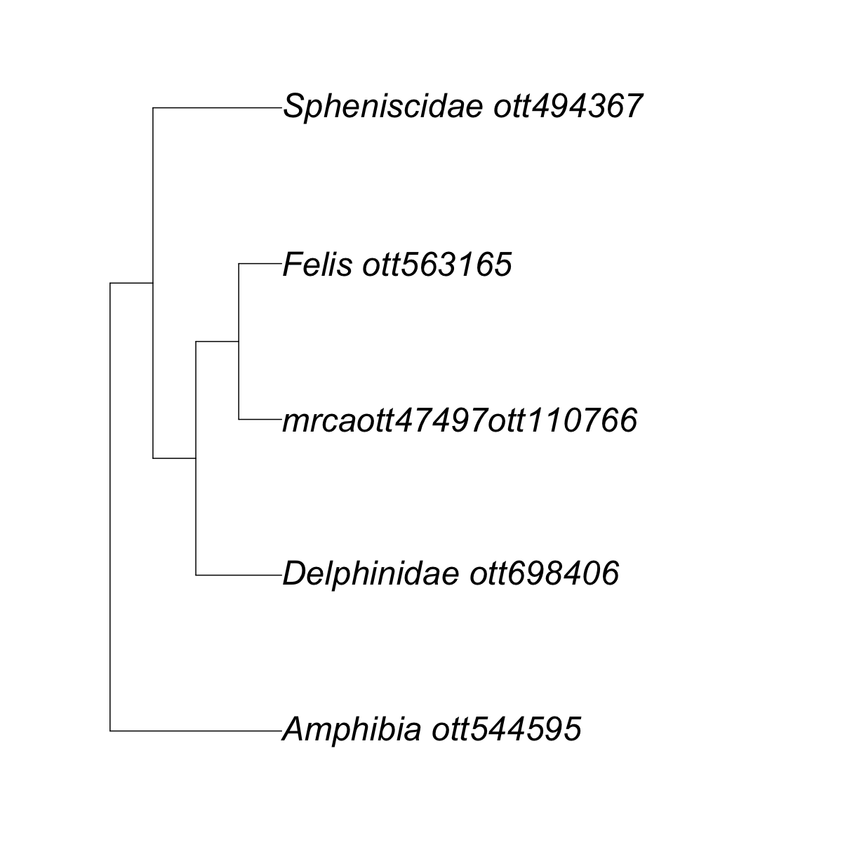
This is cool!
But, why oh why did my Canis disappear? 😢
Well, it did not actually disappear, it was replaced by the label “mrcaott47497ott110766”.
We will explain why this happens in the next section.
Now, what if you want a piece of the synthetic OpenTree containing all descendants of your taxa of interest?
Getting a subtree of one taxon
We can extract a subtree of all descendants of one taxon at a time using the function tol_subtree() and an OTT id of your choosing.
Let’s extract a subtree of all amphibians.
First, get its OTT id. It is already stored in our resolved_names object:
amphibia_ott_id <- resolved_names["Amphibia",]$ott_id
Or, you can run the function tnrs_match_names() again if you want.
amphibia_ott_id <- rotl::tnrs_match_names("amphibians")$ott_id
Now, extract the subtree from the synthetic OpenTree using tol_subtree().
amphibia_subtree <- rotl::tol_subtree(ott_id = resolved_names["Amphibia",]$ott_id)
Let’s look at the output:
amphibia_subtree
Phylogenetic tree with 10020 tips and 4669 internal nodes.

Tip labels:
  Odorrana_geminata_ott114, Odorrana_chapaensis_ott214633, Odorrana_grahami_ott43280, Odorrana_margaretae_ott440550, Odorrana_kuangwuensis_ott3618367, Odorrana_junlianensis_ott656728, ...
Node labels:
  Amphibia ott544595, Batrachia ott471197, Anura ott991547, , , , ...

Unrooted; no branch lengths.
This is a large tree! We will have a hard time plotting it.
Now, let’s extract a subtree for the genus Canis. It should be way smaller!
subtree <- rotl::tol_subtree(resolved_names["Canis",]$ott_id)
Error: HTTP failure: 400
list(contesting_trees = list(`ot_278@tree1` = list(attachment_points = list(list(children_from_taxon = list("node242"), parent = "node241"), list(children_from_taxon = list("node244"), parent = "node243"), list(children_from_taxon = list("node262"), parent = "node255"), list(children_from_taxon = list("node270"), parent = "node267"))), `ot_328@tree1` = list(attachment_points = list(list(children_from_taxon = list("node519"), parent = "node518"), list(children_from_taxon = list("node523"), parent = "node522")))),
    mrca = "mrcaott47497ott110766")[/v3/tree_of_life/subtree] Error: node_id was not found (broken taxon).
😱 😱 😱
What does this error mean??
A “broken” taxon error usually happens when phylogenetic information does not match taxonomic information.
For example, extinct lineages are sometimes phylogenetically included within a taxon but are taxonomically excluded, making the taxon appear as paraphyletic.
On the Open Tree of Life browser, we can still get to the subtree (check it out here).
From R, we will need to do something else first. We will get to that on the next episode.
Key Points
OTT ids and node ids allow us to interact with the synthetic OpenTree.
Portions of the synthetic OpenTree can be extracted from a single OTT id or from a bunch of OTT ids
It is not possible to get a subtree from an OTT id that is not in the synthetic tree.
Dealing with "broken" and "invalid" taxa
Overview
Teaching: 5 min
Exercises: 5 minQuestions
What is a broken taxon?
How do I detect it?
Objectives
Get to know the functions that interact with nodes in the synthetic OpenTree.
Understand outputs from those functions.
We say that a taxon is “broken” when its OTT id is not assigned to any node in the OpenTree synthetic tree. As mentioned before, this happens when the OTT id belongs to a taxon that is not monophyletic in the current version of the synthetic OpenTree. This is the reason why we get an error when we try to get an OpenTree synthetic subtree including the OTT id of the genus Canis –it is not monophyletic in the tree.
There is a way to find out that a group is “broken” before trying to get the subtree and getting an error.
rotl::is_in_tree(resolved_names["Canis",]$ott_id)
[1] FALSE
Indeed, our Canis is not in the synthetic OpenTree. To extract a subtree of a “broken” taxon, we have some options. But we will focus on one.
Getting the MRCA of a taxon
The function tol_node_info() gets for you all relevant information of the node that is the ancestor or MRCA of a taxon. That also includes the actual node id.
canis_node_info <- rotl::tol_node_info(resolved_names["Canis",]$ott_id)
canis_node_info
OpenTree node.

Node id: mrcaott47497ott110766
Number of terminal descendants: 85
Is taxon: FALSE
Let’s explore the class of the output.
class(canis_node_info)
[1] "tol_node" "list"
So we have an object of class ‘list’ and ‘tol_node’. When we printed it, we got some information. But we do not know how much information might not be “printed” to screen.
Let’s use the functions str() or ls() to check out the data strcture of our ‘tol_node’ object.
str(canis_node_info)
List of 8
 $ node_id      : chr "mrcaott47497ott110766"
 $ num_tips     : int 85
 $ query        : chr "ott372706"
 $ resolves     :List of 1
  ..$ pg_2812@tree6545: chr "node1135827"
 $ source_id_map:List of 5
  ..$ ot_278@tree1    :List of 3
  .. ..$ git_sha : chr ""
  .. ..$ study_id: chr "ot_278"
  .. ..$ tree_id : chr "tree1"
  ..$ ot_328@tree1    :List of 3
  .. ..$ git_sha : chr ""
  .. ..$ study_id: chr "ot_328"
  .. ..$ tree_id : chr "tree1"
  ..$ pg_1428@tree2855:List of 3
  .. ..$ git_sha : chr ""
  .. ..$ study_id: chr "pg_1428"
  .. ..$ tree_id : chr "tree2855"
  ..$ pg_2647@tree6169:List of 3
  .. ..$ git_sha : chr ""
  .. ..$ study_id: chr "pg_2647"
  .. ..$ tree_id : chr "tree6169"
  ..$ pg_2812@tree6545:List of 3
  .. ..$ git_sha : chr ""
  .. ..$ study_id: chr "pg_2812"
  .. ..$ tree_id : chr "tree6545"
 $ supported_by :List of 2
  ..$ ot_278@tree1: chr "node233"
  ..$ ot_328@tree1: chr "node495"
 $ synth_id     : chr "opentree13.4"
 $ terminal     :List of 2
  ..$ pg_1428@tree2855: chr "node610132"
  ..$ pg_2647@tree6169: chr "ott247333"
 - attr(*, "class")= chr [1:2] "tol_node" "list"
This is telling us that tol_node_info() extracted 8 different pieces of information from my node.
Right now we are only interested in the node id. Where do you think we can find it?
Hands on! Get the node id of Canis MRCA
Extract it from your
canis_node_infoobject and call itcanis_node_id.canis_node_id <- canis_node_info$node_id
Pro tip 3.1: Get the node id of the MRCA of a group of OTT ids
Sometimes you want the MRCA of a bunch of lineages. The function
tol_mrca()gets the node of the MRCA of a group of OTT ids.Can you use it to get the mrca of Canis?
The node that contains Canis is mrcaott47497ott110766.
Getting a subtree using a node id instead of the taxon OTT id
Now that we have a node id, we can use it to get a subtree with tol_subtree(), using the argument node_id.
canis_node_subtree <- rotl::tol_subtree(node_id = canis_node_id)
canis_node_subtree
Phylogenetic tree with 85 tips and 28 internal nodes.

Tip labels:
  Canis_lupus_pallipes_ott47497, Canis_lupus_chanco_ott47500, Canis_lupus_baileyi_ott67371, Canis_lupus_laniger_ott80830, Canis_lupus_hattai_ott83897, Canis_lupus_desertorum_ott234374, ...
Node labels:
  , , , , , , ...

Unrooted; no branch lengths.
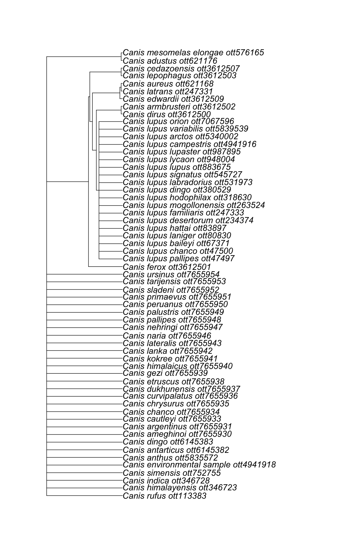
ape::plot.phylo(canis_node_subtree, cex = 1.2)
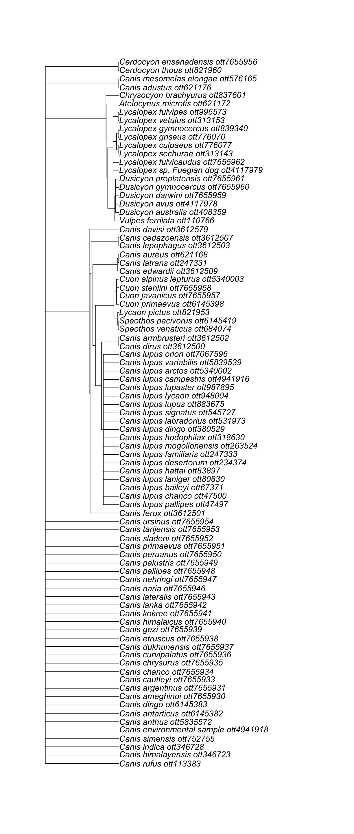
Nice! We got a subtree of 85 tips, containing all descendants from the node that also contains Canis.
If you explore the taxon names at the tip, you will notice that this includes species assigned to genera other than Canis.
Now, what if I want a subtree of certain taxonomic ranks withing my group? Go to the next episode and find out how you can do this!
Pro Tip 3.2: Get an induced subtree of taxonomic children
What if I really, really need a tree containing species within the genus Canis only, excluding everything that does not belong to the genus taxonomically, even if it does phylogenetically?
We can get the OTT ids of the taxonomic children of our taxon of interest and use the function
tol_induced_subtree().First, we will get the taxonomic children.
canis_taxonomy <- rotl::taxonomy_subtree(resolved_names["Canis",]$ott_id)canis_taxonomy$tip_label [1] "Canis_dirus_ott3612500" [2] "Canis_anthus_ott5835572" [3] "Canis_rufus_ott113383" [4] "Canis_simensis_ott752755" [5] "Canis_aureus_ott621168" [6] "Canis_mesomelas_elongae_ott576165" [7] "Canis_adustus_ott621176" [8] "unclassified_Canis_ott7655955" [9] "Canis_latrans_ott247331" [10] "Canis_lupus_baileyi_ott67371" [11] "Canis_lupus_laniger_ott80830" [12] "Canis_lupus_orion_ott7067596" [13] "Canis_lupus_hodophilax_ott318630" [14] "Canis_lupus_signatus_ott545727" [15] "Canis_lupus_arctos_ott5340002" [16] "Canis_lupus_mogollonensis_ott263524" [17] "Canis_lupus_variabilis_ott5839539" [18] "Canis_lupus_lupus_ott883675" [19] "Canis_lupus_campestris_ott4941916" [20] "Canis_lupus_lycaon_ott948004" [21] "Canis_lupus_pallipes_ott47497" [22] "Canis_lupus_chanco_ott47500" [23] "Canis_lupus_x_Canis_lupus_familiaris_ott4941915" [24] "Canis_lupus_desertorum_ott234374" [25] "Canis_lupus_familiaris_ott247333" [26] "Canis_lupus_dingo_ott380529" [27] "Canis_lupus_labradorius_ott531973" [28] "Canis_lupus_hattai_ott83897" [29] "Canis_lupus_lupaster_ott987895" [30] "Canis_himalayensis_ott346723" [31] "Canis_indica_ott346728" [32] "Canis_environmental_samples_ott4941917" [33] "Canissp.KEB-2016ott5925604" [34] "Canis_sp._CANInt1_ott470950" [35] "'Canissp.Russia/33" [36] "500ott5338950'" [37] "Canis_sp._ott247325" [38] "'Canissp.Belgium/36" [39] "000ott5338951'" [40] "Canis_environmental_sample_ott4941918" [41] "Canis_morenis_ott6145387" [42] "Canis_niger_ott6145388" [43] "Canis_palaeoplatensis_ott6145390" [44] "Canis_osorum_ott6145389" [45] "Canis_thooides_ott6145392" [46] "Canis_antarcticus_ott6145381" [47] "Canis_proplatensis_ott6145391" [48] "Canis_feneus_ott6145384" [49] "Canis_geismarianus_ott6145385" [50] "Canis_ameghinoi_ott7655930" [51] "Canis_nehringi_ott7655947" [52] "Canis_palustris_ott7655949" [53] "Canis_lanka_ott7655942" [54] "Canis_pallipes_ott7655948" [55] "Canis_gezi_ott7655939" [56] "Canis_montanus_ott7655945" [57] "Canis_primaevus_ott7655951" [58] "Canis_chrysurus_ott7655935" [59] "Canis_dukhunensis_ott7655937" [60] "Canis_kokree_ott7655941" [61] "Canis_sladeni_ott7655952" [62] "Canis_himalaicus_ott7655940" [63] "Canis_chanco_ott7655934" [64] "Canis_curvipalatus_ott7655936" [65] "Canis_lateralis_ott7655943" [66] "Canis_argentinus_ott7655931" [67] "Canis_tarijensis_ott7655953" [68] "Canis_naria_ott7655946" [69] "Canis_peruanus_ott7655950" [70] "Canis_cautleyi_ott7655933" [71] "Canis_ursinus_ott7655954" [72] "Canis_armbrusteri_ott3612502" [73] "Canis_ferox_ott3612501" [74] "Canis_lepophagus_ott3612503" [75] "Canis_edwardii_ott3612509" [76] "Canis_apolloniensis_ott3612508" [77] "Canis_cedazoensis_ott3612507" [78] "Canis_primigenius_ott3612506" [79] "Canis_lydekkeri_ott7655944" [80] "Canis_arnensis_ott7655932" [81] "Canis_antarticus_ott6145382" [82] "Canis_dingo_ott6145383" [83] "Canis_etruscus_ott7655938" [84] "Canis_spelaeus_ott3612504" $edge_label [1] "Canis_mesomelas_ott666235" "Canis_lupus_ott247341" [3] "Canis_ott372706"Now, extract the OTT ids.
canis_taxonomy_ott_ids <- datelife::extract_ott_ids(x = canis_taxonomy$tip_label)After extracting ott ids, there are some non numeric elements:Canissp.KEB-2016ott5925604 'Canissp.Russia/33 500ott5338950' 'Canissp.Belgium/36 000ott5338951'NAs removed.Try to get an induced subtree of Canis taxonomic children.
canis_taxonomy_subtree <- rotl::tol_induced_subtree(canis_taxonomy_ott_ids)Error: HTTP failure: 400 [/v3/tree_of_life/induced_subtree] Error: node_id 'ott3612504' was not found!list(ott247325 = "pruned_ott_id", ott3612504 = "pruned_ott_id", ott3612506 = "pruned_ott_id", ott3612508 = "pruned_ott_id", ott470950 = "pruned_ott_id", ott4941915 = "pruned_ott_id", ott4941917 = "pruned_ott_id", ott6145381 = "pruned_ott_id", ott6145384 = "pruned_ott_id", ott6145385 = "pruned_ott_id", ott6145387 = "pruned_ott_id", ott6145388 = "pruned_ott_id", ott6145389 = "pruned_ott_id", ott6145390 = "pruned_ott_id", ott6145391 = "pruned_ott_id", ott6145392 = "pruned_ott_id", ott7655932 = "pruned_ott_id", ott7655944 = "pruned_ott_id", ott7655945 = "pruned_ott_id", ott7655955 = "pruned_ott_id")It is often not possible to get an induced subtree of all taxonomic children from a taxon, because some of them will not make it to the synthetic tree.
To verify which ones are giving us trouble, we can use the function
is_in_tree()again.canis_in_tree <- sapply(canis_taxonomy_ott_ids, rotl::is_in_tree) # logical vector canis_taxonomy_ott_ids_intree <- canis_taxonomy_ott_ids[canis_in_tree] # extract ott ids in treeNow get the tree.
canis_taxonomy_subtree <- rotl::tol_induced_subtree(canis_taxonomy_ott_ids_intree)Plot it.
ape::plot.phylo(canis_taxonomy_subtree, cex = 1.2)
There! We have a synthetic subtree (derived from phylogenetic information) containing only the taxonomic children of Canis.
Key Points
It is not possible to get a subtre from an OTT id that is not in the synthetic tree.
OTT ids and node ids allow us to interact with the synthetic OpenTree.
Getting an induced subtree of all taxa within a taxonomic rank
Overview
Teaching: 5 min
Exercises: 5 minQuestions
How do I get all taxa from a certain taxonomic rank?
Objectives
Get an induced subtree from all taxa of a given taxonomic rank.
There is not a specific function in the package rotl that gets all taxa from a given taxonomic rank.
We will now shift to the datelife package and use the get_ott_children() function, that extracts OTT ids of all taxa from a rank specified by the argument ott_rank.
Let’s get all amphibian families.
amphibia_families <- datelife::get_ott_children(ott_ids = resolved_names["Amphibia",]$ott_id, ott_rank = "family")
str(amphibia_families)
List of 1
 $ Amphibia:'data.frame':	70 obs. of  2 variables:
  ..$ ott_id: int [1:70] 118029 639647 639653 654645 128153 114139 114359 861429 379929 4948197 ...
  ..$ rank  : chr [1:70] "family" "family" "family" "family" ...
Now, get the induced subtree using the amphibian families’ OTT ids.
amphibia_families_subtree <- rotl::tol_induced_subtree(amphibia_families$Amphibia$ott_id)
amphibia_families_subtree
Phylogenetic tree with 60 tips and 59 internal nodes.

Tip labels:
  Ranidae_ott364560, Rhacophoridae_ott432783, Mantellidae_ott38969, Ranixalidae_ott403946, Nyctibatrachidae_ott1081210, Ceratobatrachidae_ott1081207, ...
Node labels:
  Amphibia ott544595, Batrachia ott471197, Anura ott991547, mrcaott114ott3129, mrcaott114ott37876, mrcaott114ott18818, ...

Rooted; no branch lengths.
Let’s print the output.
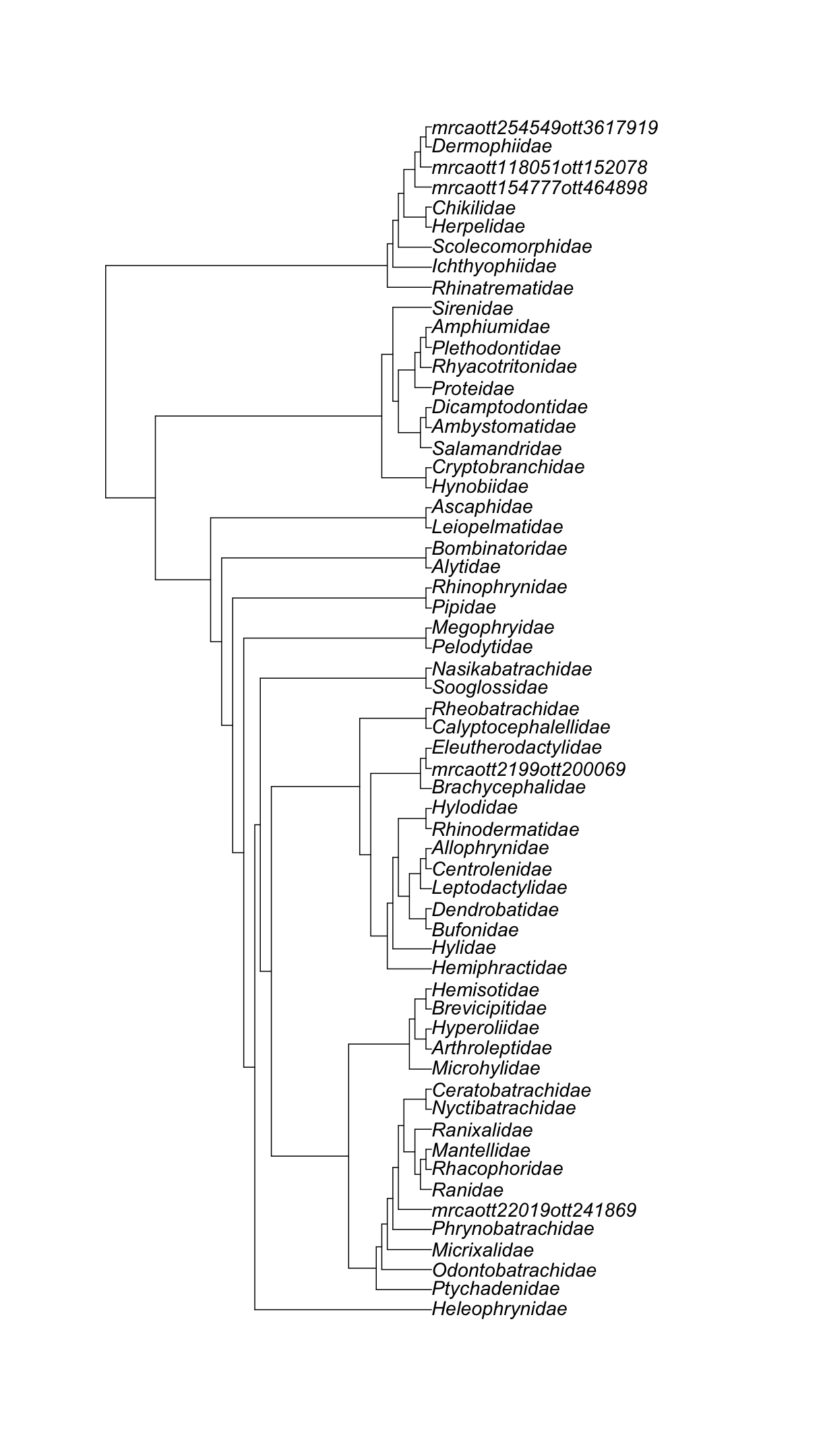
ape::plot.phylo(amphibia_families_subtree, cex = 1.2)
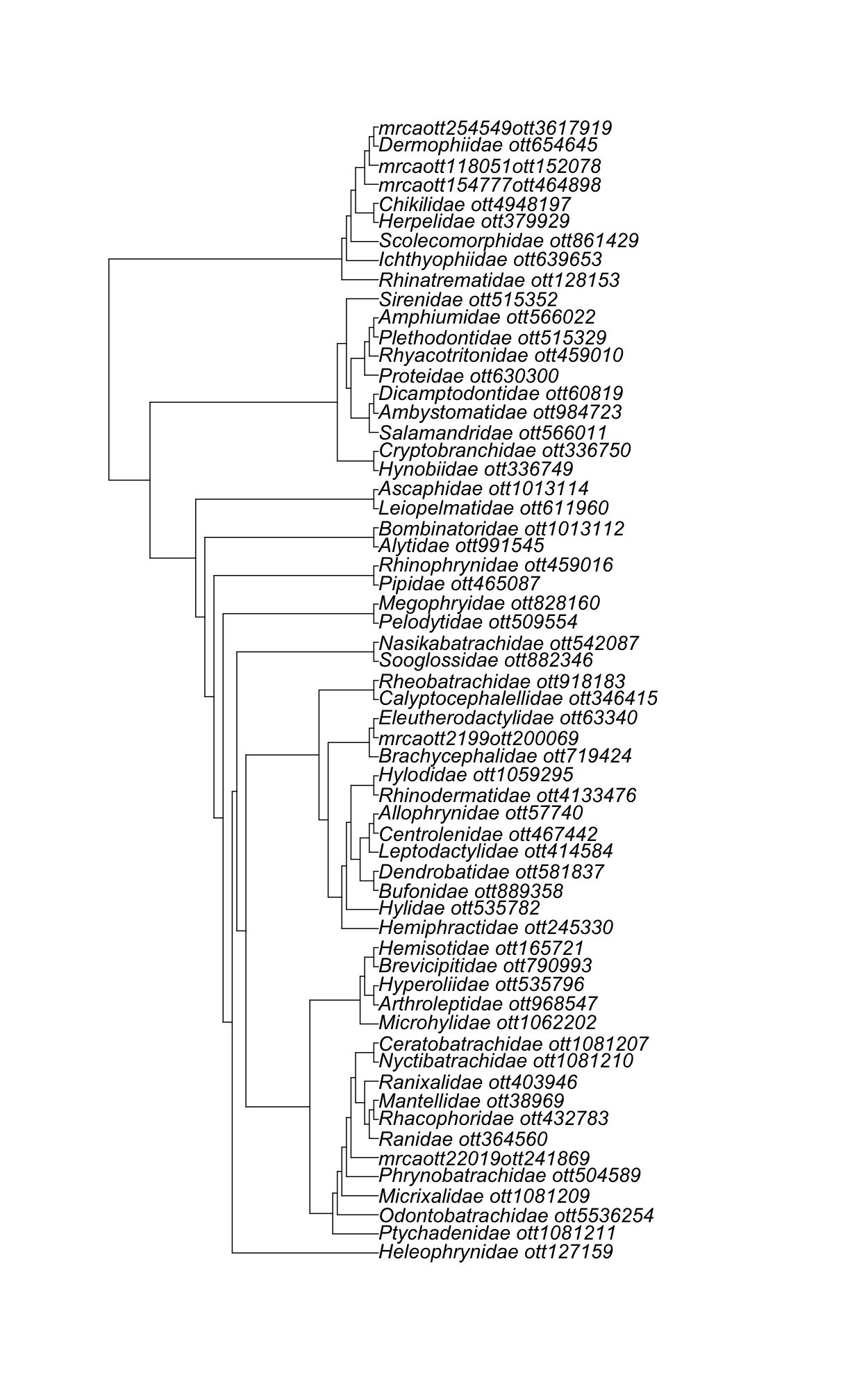
Super cool!
Hands on! Get a family subtree without ott ids in the tip labels
Hint: Look at the arguments of function
tol_induced_subtree()Solution
amphibia_families_subtree2 <- rotl::tol_induced_subtree(amphibia_families$Amphibia$ott_id, label_format = "name")Warning in collapse_singles(tr, show_progress): Dropping singleton nodes with labels: mrcaott114ott391676, mrcaott15857ott152667, mrcaott270630ott3618180, mrcaott22583ott100573, mrcaott22583ott44382, mrcaott44382ott72638, mrcaott44382ott100564, mrcaott65695ott254163, mrcaott65695ott121259, mrcaott2199ott411156, mrcaott7464ott21502, mrcaott21502ott918196, Pelobatoidea, mrcaott18818ott47772, Sirenoideaape::plot.phylo(amphibia_families_subtree2, cex = 1.2)
We have seen up to now how to get a portion of the synthetic OpenTree. How do I inspect the source phylogenetic trees that support the subtrees?
Pro Tip 4.1: Get all taxa from a taxonomic rank.
While
datelifefacilitates this task, there are other ways to get all taxa from a taxonmic rank using mostlyrotlfunctions. Try it out!amphibia_taxonomy <- rotl::taxonomy_subtree(resolved_names["Amphibia",]$ott_id[[1]]) ls(amphibia_taxonomy) length(amphibia_taxonomy$tip_label) head(amphibia_taxonomy$tip_label) tail(amphibia_taxonomy$tip_label) amphibia_taxonomy$edge_label edges <- datelife::extract_ott_ids(x=amphibia_taxonomy$edge_label) length(edges) # The following line takes a while to run! edges_taxon_info <- rotl::taxonomy_taxon_info(edges) ls(edges_taxon_info[[1]]) is_family <- unname(unlist(sapply(edges_taxon_info, "[", "rank") %in% "family")) is_suppressed <- unname(unlist(sapply(edges_taxon_info, "[", "is_suppressed_from_synth"))) # flag "is suppressed from synth" is not updated, so it is useless for now. amphibia_families <- unname(unlist(sapply(edges_taxon_info, "[", "ott_id")[is_family])) in_tree <- rotl::is_in_tree(amphibia_families) amphibia_families_subtree <- rotl::tol_induced_subtree(amphibia_families[in_tree])
Key Points
It is possible to get all types of subsets from the synthetic tree, as long as you can get the OTT ids!
Getting studies and trees supporting relationships in a synthetic subtree
Overview
Teaching: 5 min
Exercises: 5 minQuestions
What are the original studies supporting relationships in my synthetic subtree?
Objectives
Get supporting trees for certain regions of the synthetic OpenTree.
To get the source trees supporting a node from our OpenTree synthetic subtree we will need two functions.
The function source_list() gets the study and tree ids (and other info) from source studies (not the trees). It is applied to a ‘tol_node’ object.
We already have one that we generated with tol_node_info(), do you remember how we called it?
Hands on! Get all supporting trees.
Get the supporting study metadata from the Canis node info. Store it in an object called
canis_node_studies. Look at its class and the information it contains.canis_node_studies <- rotl::source_list(canis_node_info)class(canis_node_studies)[1] "data.frame"str(canis_node_studies)'data.frame': 5 obs. of 3 variables: $ study_id: chr "ot_278" "ot_328" "pg_1428" "pg_2647" ... $ tree_id : chr "tree1" "tree1" "tree2855" "tree6169" ... $ git_sha : chr "" "" "" "" ...
Now that we have the ids, we can use the function get_study_tree(), which will get us the actual supporting trees.
This function takes one study id and tree id at a time, like this:
index <- 1

rotl::get_study_tree(study_id = canis_node_studies$study_id[index], tree_id = canis_node_studies$tree_id[index], tip_label="ott_taxon_name", deduplicate = TRUE)
Warning: Some tip labels were duplicated and have been modified: Leptocyon,
Leptocyon, Leptocyon, Leptocyon, Leptocyon, Leptocyon, Leptocyon, Canidae,
Canidae, Urocyon, Urocyon, Urocyon, Cerdocyon, Canis, Canis, Canis, Canis,
Canis, Canis, Canis, Canis, Canis, Canidae, Cynarctoides
Phylogenetic tree with 142 tips and 141 internal nodes.

Tip labels:
  Prohesperocyon_wilsoni, Ectopocynus_antiquus, Ectopocynus_intermedius, Ectopocynus_simplicidens, Hesperocyon, Hesperocyon_gregarius, ...

Rooted; includes branch lengths.
Hands on! Get all supporting trees.
Call the output canis_source_trees
Hint: You can use a “for” loop or an
apply()function to get them all.Solution
With a ‘for’ loop.
canis_source_trees <- vector(mode = "list") # generate an empty list
for (i in seq(nrow(canis_node_studies))){
  source_tree <- rotl::get_study_tree(study_id = canis_node_studies$study_id[i], tree_id = canis_node_studies$tree_id[i], tip_label="ott_taxon_name", deduplicate = TRUE)
  canis_source_trees <- c(canis_source_trees, list(source_tree))
}
Warning: Some tip labels were duplicated and have been modified: Leptocyon, Leptocyon, Leptocyon, Leptocyon, Leptocyon, Leptocyon, Leptocyon, Canidae, Canidae, Urocyon, Urocyon, Urocyon, Cerdocyon, Canis, Canis, Canis, Canis, Canis, Canis, Canis, Canis, Canis, Canidae, Cynarctoidescanis_source_trees[[1]] Phylogenetic tree with 142 tips and 141 internal nodes. Tip labels: Prohesperocyon_wilsoni, Ectopocynus_antiquus, Ectopocynus_intermedius, Ectopocynus_simplicidens, Hesperocyon, Hesperocyon_gregarius, ... Rooted; includes branch lengths. [[2]] Phylogenetic tree with 294 tips and 272 internal nodes. Tip labels: Homo_sapiens, Rattus_norvegicus, Mus_musculus, Artibeus_jamaicensis, Mystacina_tuberculata, Tadarida_brasiliensis, ... Rooted; includes branch lengths. [[3]] Phylogenetic tree with 169 tips and 168 internal nodes. Tip labels: Xenopus_laevis, Anolis_carolinensis, Gallus_gallus, Taeniopygia_guttata, Tachyglossus_aculeatus, Ornithorhynchus_anatinus, ... Rooted; includes branch lengths. [[4]] Phylogenetic tree with 86 tips and 85 internal nodes. Tip labels: *tip_#1_not_mapped_to_OTT._Original_label_-_Morganucodon_oehleri, *tip_#2_not_mapped_to_OTT._Original_label_-_Morganucodon_watsoni, *tip_#3_not_mapped_to_OTT._Original_label_-_Haldanodon_exspectatus, Eomaia_scansoria, Amblysomus_hottentotus, Echinops_telfairi, ... Rooted; no branch lengths. [[5]] Phylogenetic tree with 78 tips and 77 internal nodes. Tip labels: Ornithorhynchus, Manis, Ailuropoda, Canis, Felis, Panthera, ... Rooted; no branch lengths.With an
apply()function.canis_source_trees <- sapply(seq(nrow(canis_node_studies)), function(i) rotl::get_study_tree(study_id = canis_node_studies$study_id[i], tree_id = canis_node_studies$tree_id[i], tip_label="ott_taxon_name", deduplicate = TRUE))Warning: Some tip labels were duplicated and have been modified: Leptocyon, Leptocyon, Leptocyon, Leptocyon, Leptocyon, Leptocyon, Leptocyon, Canidae, Canidae, Urocyon, Urocyon, Urocyon, Cerdocyon, Canis, Canis, Canis, Canis, Canis, Canis, Canis, Canis, Canis, Canidae, Cynarctoidescanis_source_trees[[1]] Phylogenetic tree with 142 tips and 141 internal nodes. Tip labels: Prohesperocyon_wilsoni, Ectopocynus_antiquus, Ectopocynus_intermedius, Ectopocynus_simplicidens, Hesperocyon, Hesperocyon_gregarius, ... Rooted; includes branch lengths. [[2]] Phylogenetic tree with 294 tips and 272 internal nodes. Tip labels: Homo_sapiens, Rattus_norvegicus, Mus_musculus, Artibeus_jamaicensis, Mystacina_tuberculata, Tadarida_brasiliensis, ... Rooted; includes branch lengths. [[3]] Phylogenetic tree with 169 tips and 168 internal nodes. Tip labels: Xenopus_laevis, Anolis_carolinensis, Gallus_gallus, Taeniopygia_guttata, Tachyglossus_aculeatus, Ornithorhynchus_anatinus, ... Rooted; includes branch lengths. [[4]] Phylogenetic tree with 86 tips and 85 internal nodes. Tip labels: *tip_#1_not_mapped_to_OTT._Original_label_-_Morganucodon_oehleri, *tip_#2_not_mapped_to_OTT._Original_label_-_Morganucodon_watsoni, *tip_#3_not_mapped_to_OTT._Original_label_-_Haldanodon_exspectatus, Eomaia_scansoria, Amblysomus_hottentotus, Echinops_telfairi, ... Rooted; no branch lengths. [[5]] Phylogenetic tree with 78 tips and 77 internal nodes. Tip labels: Ornithorhynchus, Manis, Ailuropoda, Canis, Felis, Panthera, ... Rooted; no branch lengths.
The object canis_node_studies contains a lot of information. You can get it using a ‘for’ loop, or an apply() function.
A key piece of information are the citations from the supporting studies. We can get these for each source trees with the function get_study_meta(). Let’s do it. First we need the study meta:
canis_node_studies_meta <- lapply(seq(nrow(canis_node_studies)), function(i)
  rotl::get_study_meta(study_id = canis_node_studies$study_id[i]))
Now we can get the citations:
canis_node_studies_citations <- sapply(seq(length(canis_node_studies_meta)), function (i) canis_node_studies_meta[[i]]$nexml$`^ot:studyPublicationReference`)
Finally, let’s plot the supporting trees along with their citations.
for (i in seq(length(canis_source_trees))){
  print(paste("The supporting tree below has", length(canis_source_trees[[i]]$tip.label), "tips."))
  print(paste("Citation is:", canis_node_studies_citations[i]))
  ape::plot.phylo(canis_source_trees[[i]])
}
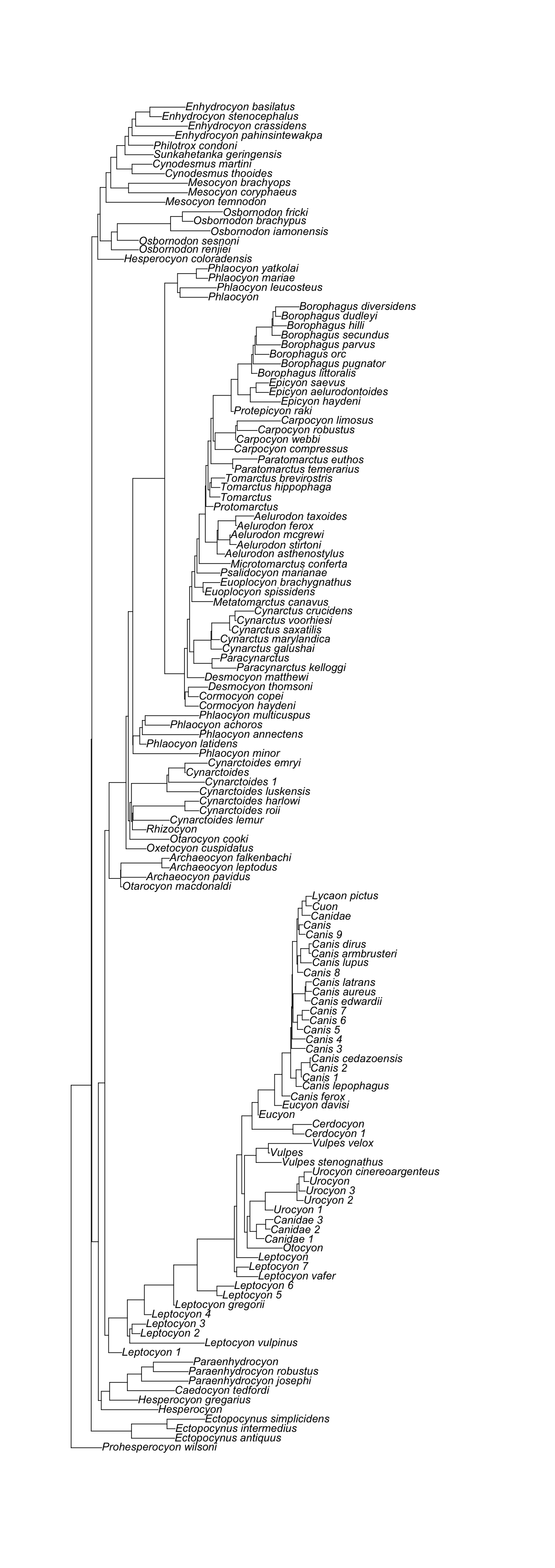
[1] "The supporting tree below has 142 tips."
[1] "Citation is: Tedford, Richard H.; Wang, Xiaoming; Taylor, Beryl E. (2009). Phylogenetic systematics of the North American fossil Caninae (Carnivora, Canidae). Bulletin of the American Museum of Natural History, no. 325. http://hdl.handle.net/2246/5999\n\nWang, Xiaoming; Tedford, Richard H.; Taylor, Beryl E. (1999). Phylogenetic systematics of the Borophaginae (Carnivora, Canidae). Bulletin of the American Museum of Natural History, no. 243. http://hdl.handle.net/2246/1588\n\nWang, Xiaoming (1994). Phylogenetic systematics of the Hesperocyoninae (Carnivora, Canidae). Bulletin of the  American Museum of Natural History, no. 221. http://hdl.handle.net/2246/829\n"
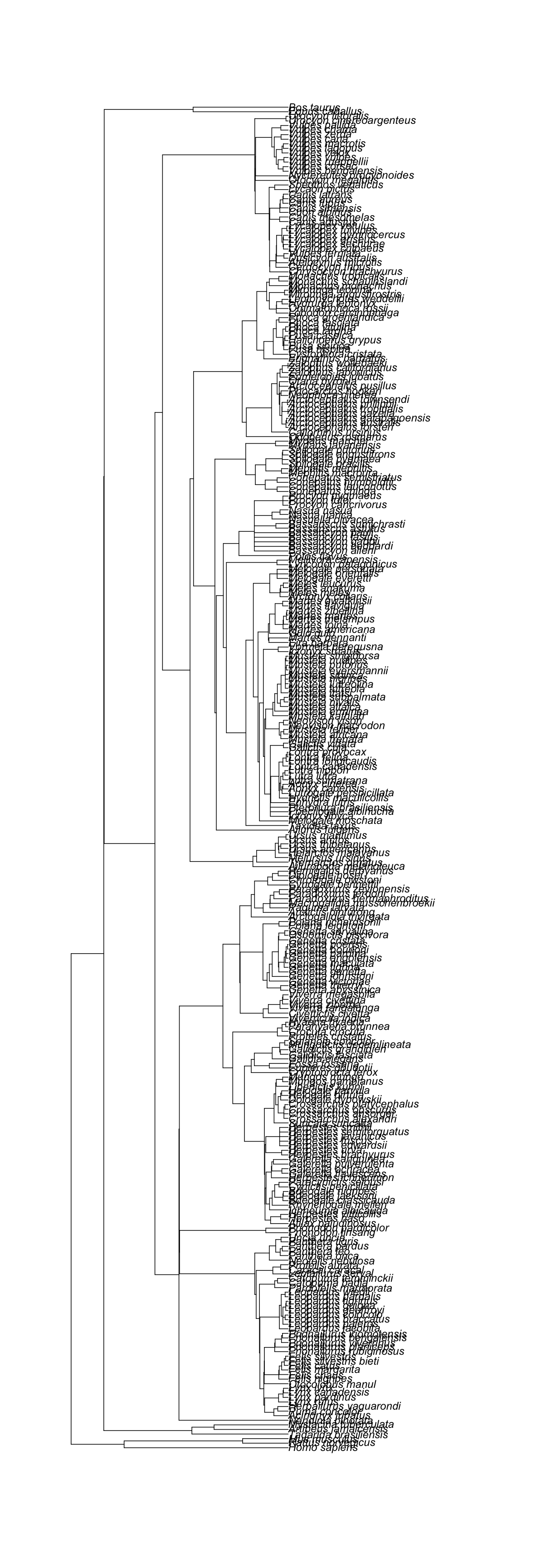
[1] "The supporting tree below has 294 tips."
[1] "Citation is: Nyakatura, Katrin, Olaf RP Bininda-Emonds. 2012. Updating the evolutionary history of Carnivora (Mammalia): a new species-level supertree complete with divergence time estimates. BMC Biology 10 (1): 12"
[1] "The supporting tree below has 169 tips."
[1] "Citation is: Meredith, R.W., Janecka J., Gatesy J., Ryder O.A., Fisher C., Teeling E., Goodbla A., Eizirik E., Simao T., Stadler T., Rabosky D., Honeycutt R., Flynn J., Ingram C., Steiner C., Williams T., Robinson T., Herrick A., Westerman M., Ayoub N., Springer M., & Murphy W. 2011. Impacts of the Cretaceous Terrestrial Revolution and KPg Extinction on Mammal Diversification. Science 334 (6055): 521-524."
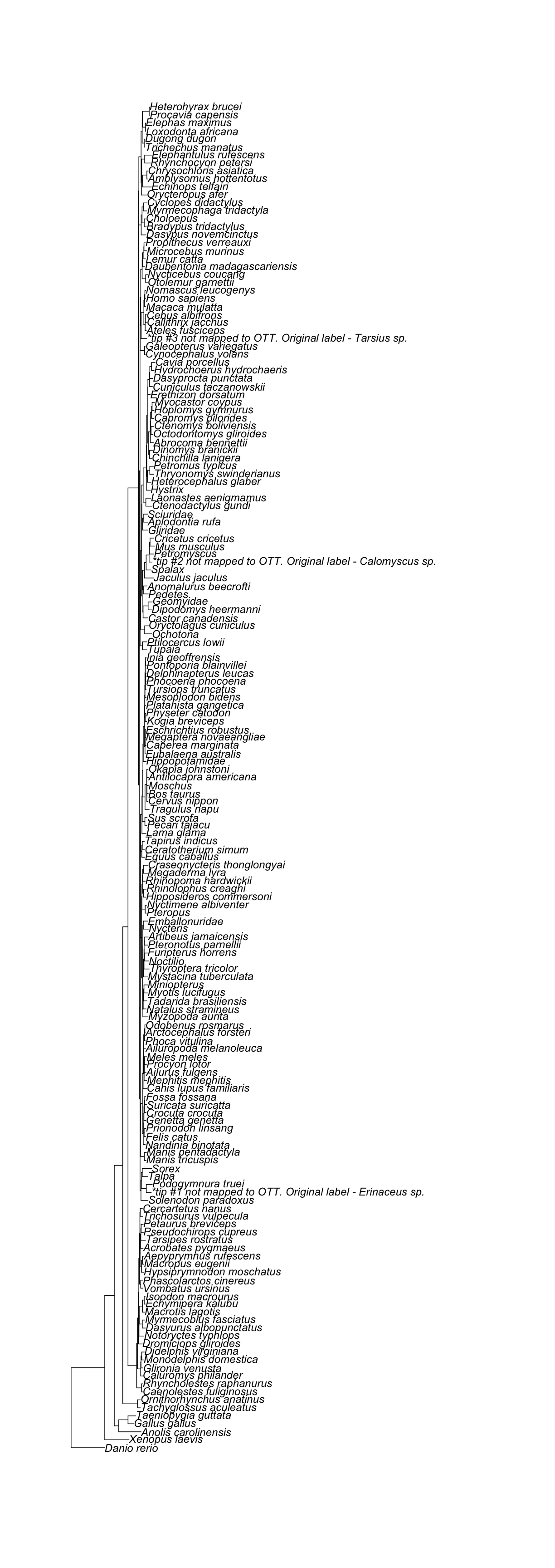
[1] "The supporting tree below has 86 tips."
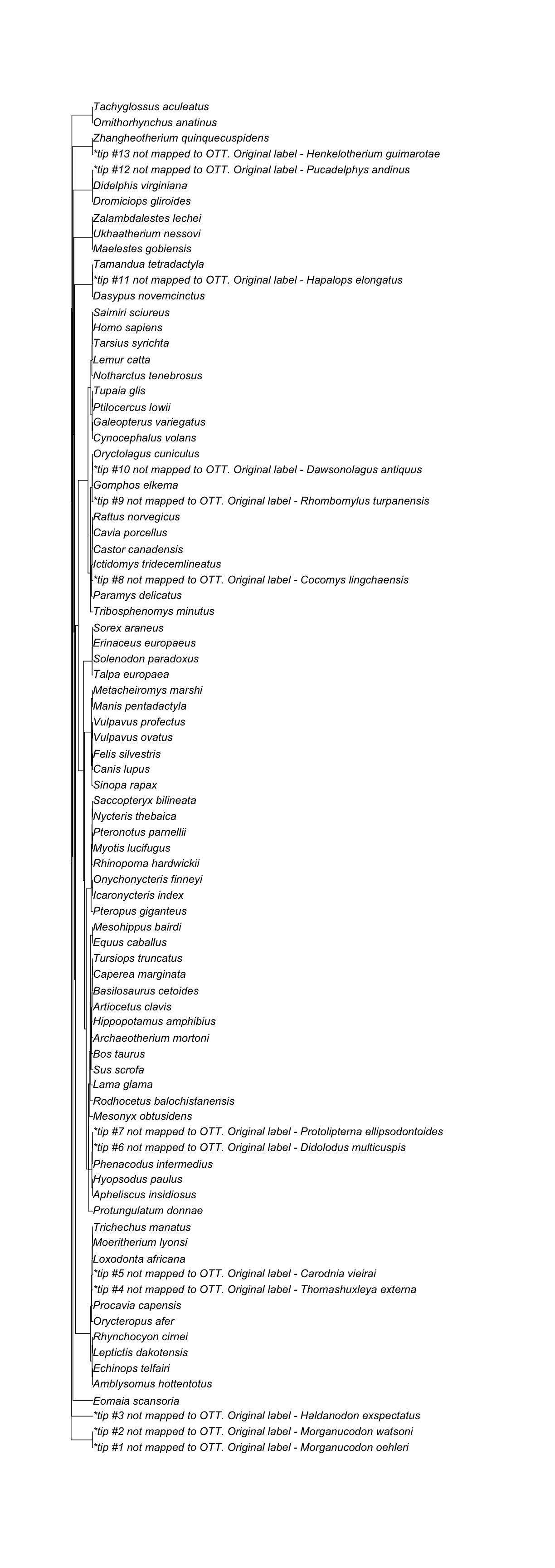
[1] "Citation is: O'Leary, M. A., J. I. Bloch, J. J. Flynn, T. J. Gaudin, A. Giallombardo, N. P. Giannini, S. L. Goldberg, B. P. Kraatz, Z.-X. Luo, J. Meng, X. Ni, M. J. Novacek, F. A. Perini, Z. S. Randall, G. W. Rougier, E. J. Sargis, M. T. Silcox, N. B. Simmons, M. Spaulding, P. M. Velazco, M. Weksler, J. R. Wible, A. L. Cirranello. 2013. The placental mammal ancestor and the post-K-Pg radiation of placentals. Science 339 (6120): 662-667."
[1] "The supporting tree below has 78 tips."
[1] "Citation is: Lartillot, Nicolas, Frédéric Delsuc. 2012. Joint reconstruction of divergence times and life-history evolution in placental mammals using a phylogenetic covariance model. Evolution 66 (6): 1773-1787."
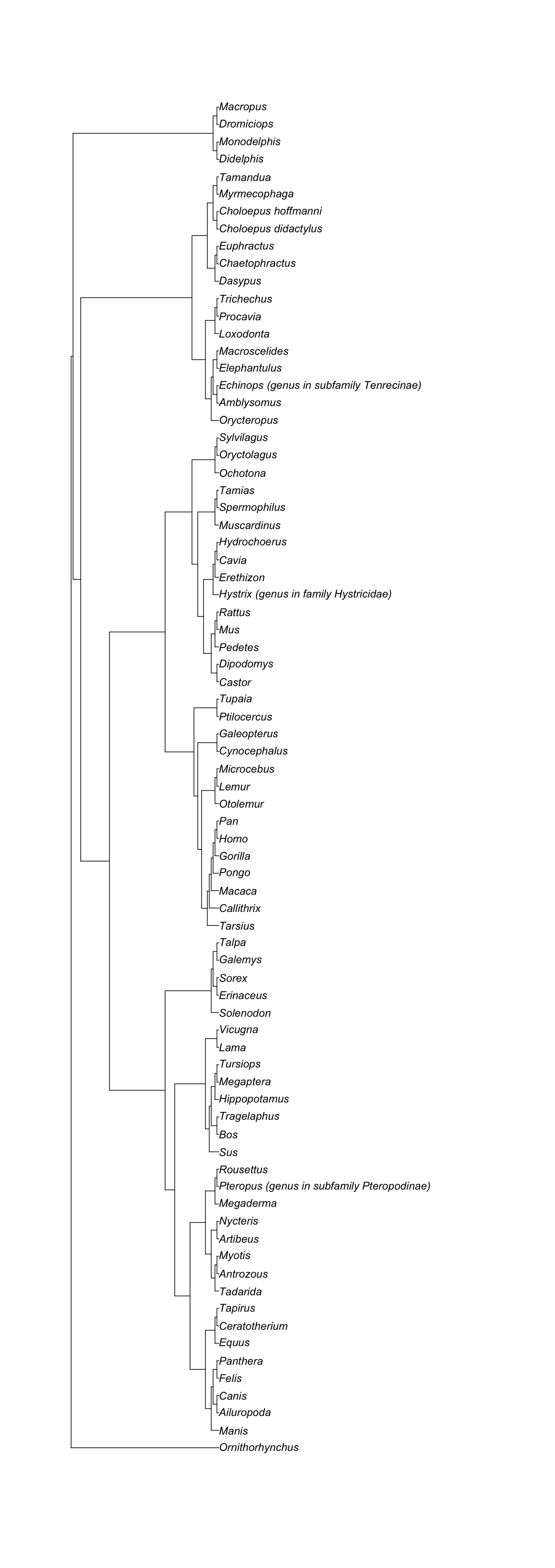
Note that the supporting trees for a node can be larger than the subtree itself.
You will have to drop the unwanted taxa from the supporting studies if you just want the parts that belong to the subtree.
Moreover, the tip labels have different taxon names in the source trees and the OpenTree synthetic subtrees. I you go to the browser, you can access original tips and matched tips, but R drops that info. We would have to standardize them with TNRS before trying to subset, and that takes some time and often visual inspection.
Key Points
Supporting trees usually contain more taxa than the ones we are interested in.
Getting branch length information (proportional to time) for you taxa
Overview
Teaching: 5 min
Exercises: 5 minQuestions
How do I find supporting trees that include branch lengths?
How do I subset them to include just the taxa I am interested in?
Objectives
Learn about the
opentree_chronogramsobject from datelife.Get source chronograms from the
opentree_chronogramsobject for a set of taxa.
What if I want to search the OpenTree database (Phylesystem) for studies and trees matching some criteria?
The rotl package has functions that allow getting a list of studies or source trees matching specific criteria.
You will recognise these functions because they start with the word studies_.
Now, what kind of properties can we search for in the OpenTree database?
The function studies_properties() gets for us two lists, one for studies and another one for tree properties available for search.
Take a look at them:
rotl::studies_properties()
$study_properties
 [1] "dc:subject"                    "dc:date"
 [3] "ot:messages"                   "dc:title"
 [5] "skos:changeNote"               "ot:studyPublicationReference"
 [7] "ot:candidateTreeForSynthesis"  "ot:taxonLinkPrefixes"
 [9] "treebaseId"                    "ot:focalCladeOTTTaxonName"
[11] "prism:modificationDate"        "dc:contributor"
[13] "dc:creator"                    "xmlns"
[15] "ot:curatorName"                "prism:number"
[17] "tb:identifier.study.tb1"       "id"
[19] "ot:otusElementOrder"           "ot:dataDeposit"
[21] "skos:historyNote"              "ot:treesElementOrder"
[23] "prism:endingPage"              "prism:section"
[25] "nexml2json"                    "ot:notIntendedForSynthesis"
[27] "ntrees"                        "treesById"
[29] "about"                         "prism:publicationName"
[31] "tb:identifier.study"           "ot:studyYear"
[33] "otusById"                      "nexmljson"
[35] "ot:annotationEvents"           "prism:doi"
[37] "ot:studyId"                    "prism:pageRange"
[39] "dc:publisher"                  "ot:studyPublication"
[41] "prism:volume"                  "tb:title.study"
[43] "ot:agents"                     "generator"
[45] "prism:publicationDate"         "ot:tag"
[47] "ot:comment"                    "ot:focalClade"
[49] "prism:startingPage"            "xhtml:license"
[51] "prism:creationDate"            "version"
[53] "dcterms:bibliographicCitation"

$tree_properties
 [1] "ot:messages"                      "xsi:type"
 [3] "ot:nearestTaxonMRCAName"          "meta"
 [5] "ot:specifiedRoot"                 "ot:reasonsToExcludeFromSynthesis"
 [7] "tb:quality.tree"                  "ot:branchLengthTimeUnit"
 [9] "ot:nodeLabelMode"                 "ot:rootNodeId"
[11] "ot:inGroupClade"                  "ot:ottTaxonName"
[13] "ot:branchLengthDescription"       "ot:studyId"
[15] "ot:MRCAName"                      "ot:unrootedTree"
[17] "tb:kind.tree"                     "tb:type.tree"
[19] "edgeBySourceId"                   "ot:nodeLabelDescription"
[21] "nodeById"                         "ot:curatedType"
[23] "ot:nearestTaxonMRCAOttId"         "ot:tag"
[25] "rootedge"                         "label"
[27] "ntips"                            "tb:ntax.tree"
[29] "ot:ottId"                         "ot:nodeLabelTimeUnit"
[31] "ot:outGroupEdge"                  "ot:branchLengthMode"
[33] "ot:MRCAOttId"
As you can see, the actual values that this properties can take are not available in the output of the function. Go to the phylesystem API wiki to get them, along with an explanation of their meaning.
To get all trees with branch lengths poprotional to time we need the function
studies_find_trees(), using the property “ot:branchLengthMode” and the value “ot:time”.
It takes some time for it to get all the information, so we will not do it now.
Go to Instructor Notes later for more information on how to do this.
Search the OpenTree chronogram database using datelife
In the package datelife, we have implemented a workflow that extracts all studies containing information from at least two taxa.
You can get all source chronograms from an induced subtree, as long as the tip labels are in the “name” format (and not the default “name_and_id”).
datelife takes as input either a tree with tip labels as scientific names (andd not names and ids), or a vector of scientific names.
Get a Canis subtree with tip labels that do not contain the OTT id.
canis_node_subtree <- rotl::tol_subtree(node_id = canis_node_info$node_id, label = "name")
canis_node_subtree
Phylogenetic tree with 85 tips and 28 internal nodes.

Tip labels:
  Canis_lupus_pallipes, Canis_lupus_chanco, Canis_lupus_baileyi, Canis_lupus_laniger, Canis_lupus_hattai, Canis_lupus_desertorum, ...
Node labels:
  , , , , , , ...

Unrooted; no branch lengths.
Now, you can use that tree as input for the get_datelife_result() function.
canis_dr <- datelife::get_datelife_result(canis_node_subtree)
Running 'make_datelife_query'...
We have now a list of matrices storing time of lineage divergence data for all taxon pairs.
Lists are named with the study citation, so we have that information handy at all times.
Let’s explore the output.
names(canis_dr)
[1] "Bininda-Emonds, Olaf R. P., Marcel Cardillo, Kate E. Jones, Ross D. E. MacPhee, Robin M. D. Beck, Richard Grenyer, Samantha A. Price, Rutger A. Vos, John L. Gittleman, Andy Purvis. 2007. The delayed rise of present-day mammals. Nature 446 (7135): 507-512"
[2] "Bininda-Emonds, Olaf R. P., Marcel Cardillo, Kate E. Jones, Ross D. E. MacPhee, Robin M. D. Beck, Richard Grenyer, Samantha A. Price, Rutger A. Vos, John L. Gittleman, Andy Purvis. 2007. The delayed rise of present-day mammals. Nature 446 (7135): 507-512"
[3] "Bininda-Emonds, Olaf R. P., Marcel Cardillo, Kate E. Jones, Ross D. E. MacPhee, Robin M. D. Beck, Richard Grenyer, Samantha A. Price, Rutger A. Vos, John L. Gittleman, Andy Purvis. 2007. The delayed rise of present-day mammals. Nature 446 (7135): 507-512"
[4] "Nyakatura, Katrin, Olaf RP Bininda-Emonds. 2012. Updating the evolutionary history of Carnivora (Mammalia): a new species-level supertree complete with divergence time estimates. BMC Biology 10 (1): 12"
[5] "Nyakatura, Katrin, Olaf RP Bininda-Emonds. 2012. Updating the evolutionary history of Carnivora (Mammalia): a new species-level supertree complete with divergence time estimates. BMC Biology 10 (1): 12"
[6] "Nyakatura, Katrin, Olaf RP Bininda-Emonds. 2012. Updating the evolutionary history of Carnivora (Mammalia): a new species-level supertree complete with divergence time estimates. BMC Biology 10 (1): 12"
[7] "Hedges, S. Blair, Julie Marin, Michael Suleski, Madeline Paymer, Sudhir Kumar. 2015. Tree of life reveals clock-like speciation and diversification. Molecular Biology and Evolution 32 (4): 835-845"
canis_dr[1] # look at the first element of the list
$`Bininda-Emonds, Olaf R. P., Marcel Cardillo, Kate E. Jones, Ross D. E. MacPhee, Robin M. D. Beck, Richard Grenyer, Samantha A. Price, Rutger A. Vos, John L. Gittleman, Andy Purvis. 2007. The delayed rise of present-day mammals. Nature 446 (7135): 507-512`
                      Canis rufus Canis latrans Canis simensis Canis adustus
Canis rufus                   0.0           2.8            2.8           3.2
Canis latrans                 2.8           0.0            2.8           3.2
Canis simensis                2.8           2.8            0.0           3.2
Canis adustus                 3.2           3.2            3.2           0.0
Canis aureus                  3.2           3.2            3.2           2.6
Lycalopex culpaeus            6.4           6.4            6.4           6.4
Lycalopex griseus             6.4           6.4            6.4           6.4
Lycalopex gymnocercus         6.4           6.4            6.4           6.4
Lycalopex sechurae            6.4           6.4            6.4           6.4
Lycalopex vetulus             6.4           6.4            6.4           6.4
Atelocynus microtis           6.4           6.4            6.4           6.4
Cerdocyon thous               6.4           6.4            6.4           6.4
Chrysocyon brachyurus         6.4           6.4            6.4           6.4
Lycaon pictus                 6.4           6.4            6.4           6.4
Speothos venaticus            6.4           6.4            6.4           6.4
Vulpes ferrilata             14.8          14.8           14.8          14.8
                      Canis aureus Lycalopex culpaeus Lycalopex griseus
Canis rufus                    3.2                6.4               6.4
Canis latrans                  3.2                6.4               6.4
Canis simensis                 3.2                6.4               6.4
Canis adustus                  2.6                6.4               6.4
Canis aureus                   0.0                6.4               6.4
Lycalopex culpaeus             6.4                0.0               1.0
Lycalopex griseus              6.4                1.0               0.0
Lycalopex gymnocercus          6.4                1.0               1.0
Lycalopex sechurae             6.4                1.0               1.0
Lycalopex vetulus              6.4                1.4               1.4
Atelocynus microtis            6.4                6.4               6.4
Cerdocyon thous                6.4                6.4               6.4
Chrysocyon brachyurus          6.4                6.4               6.4
Lycaon pictus                  6.4                6.4               6.4
Speothos venaticus             6.4                6.4               6.4
Vulpes ferrilata              14.8               14.8              14.8
                      Lycalopex gymnocercus Lycalopex sechurae
Canis rufus                             6.4                6.4
Canis latrans                           6.4                6.4
Canis simensis                          6.4                6.4
Canis adustus                           6.4                6.4
Canis aureus                            6.4                6.4
Lycalopex culpaeus                      1.0                1.0
Lycalopex griseus                       1.0                1.0
Lycalopex gymnocercus                   0.0                1.0
Lycalopex sechurae                      1.0                0.0
Lycalopex vetulus                       1.4                1.4
Atelocynus microtis                     6.4                6.4
Cerdocyon thous                         6.4                6.4
Chrysocyon brachyurus                   6.4                6.4
Lycaon pictus                           6.4                6.4
Speothos venaticus                      6.4                6.4
Vulpes ferrilata                       14.8               14.8
                      Lycalopex vetulus Atelocynus microtis Cerdocyon thous
Canis rufus                         6.4                 6.4             6.4
Canis latrans                       6.4                 6.4             6.4
Canis simensis                      6.4                 6.4             6.4
Canis adustus                       6.4                 6.4             6.4
Canis aureus                        6.4                 6.4             6.4
Lycalopex culpaeus                  1.4                 6.4             6.4
Lycalopex griseus                   1.4                 6.4             6.4
Lycalopex gymnocercus               1.4                 6.4             6.4
Lycalopex sechurae                  1.4                 6.4             6.4
Lycalopex vetulus                   0.0                 6.4             6.4
Atelocynus microtis                 6.4                 0.0             6.4
Cerdocyon thous                     6.4                 6.4             0.0
Chrysocyon brachyurus               6.4                 6.4             6.4
Lycaon pictus                       6.4                 6.4             6.4
Speothos venaticus                  6.4                 6.4             6.4
Vulpes ferrilata                   14.8                14.8            14.8
                      Chrysocyon brachyurus Lycaon pictus Speothos venaticus
Canis rufus                             6.4           6.4                6.4
Canis latrans                           6.4           6.4                6.4
Canis simensis                          6.4           6.4                6.4
Canis adustus                           6.4           6.4                6.4
Canis aureus                            6.4           6.4                6.4
Lycalopex culpaeus                      6.4           6.4                6.4
Lycalopex griseus                       6.4           6.4                6.4
Lycalopex gymnocercus                   6.4           6.4                6.4
Lycalopex sechurae                      6.4           6.4                6.4
Lycalopex vetulus                       6.4           6.4                6.4
Atelocynus microtis                     6.4           6.4                6.4
Cerdocyon thous                         6.4           6.4                6.4
Chrysocyon brachyurus                   0.0           6.4                6.4
Lycaon pictus                           6.4           0.0                6.4
Speothos venaticus                      6.4           6.4                0.0
Vulpes ferrilata                       14.8          14.8               14.8
                      Vulpes ferrilata
Canis rufus                       14.8
Canis latrans                     14.8
Canis simensis                    14.8
Canis adustus                     14.8
Canis aureus                      14.8
Lycalopex culpaeus                14.8
Lycalopex griseus                 14.8
Lycalopex gymnocercus             14.8
Lycalopex sechurae                14.8
Lycalopex vetulus                 14.8
Atelocynus microtis               14.8
Cerdocyon thous                   14.8
Chrysocyon brachyurus             14.8
Lycaon pictus                     14.8
Speothos venaticus                14.8
Vulpes ferrilata                   0.0
canis_dr[length(canis_dr)] # look at the last element of the list
$`Hedges, S. Blair, Julie Marin, Michael Suleski, Madeline Paymer, Sudhir Kumar. 2015. Tree of life reveals clock-like speciation and diversification. Molecular Biology and Evolution 32 (4): 835-845`
                      Chrysocyon brachyurus Lycaon pictus Speothos venaticus
Chrysocyon brachyurus               0.00000      13.58235           13.58235
Lycaon pictus                      13.58235       0.00000           10.91794
Speothos venaticus                 13.58235      10.91794            0.00000
Lycalopex vetulus                  16.55066      16.55066           16.55066
Lycalopex fulvipes                 16.55066      16.55066           16.55066
Lycalopex culpaeus                 16.55066      16.55066           16.55066
Lycalopex gymnocercus              16.55066      16.55066           16.55066
Lycalopex griseus                  16.55066      16.55066           16.55066
Lycalopex sechurae                 16.55066      16.55066           16.55066
Cerdocyon thous                    16.55066      16.55066           16.55066
Atelocynus microtis                16.55066      16.55066           16.55066
Canis adustus                      16.55066      16.55066           16.55066
Canis latrans                      16.55066      16.55066           16.55066
Canis aureus                       16.55066      16.55066           16.55066
Canis simensis                     16.55066      16.55066           16.55066
Dusicyon australis                 18.25725      18.25725           18.25725
Vulpes ferrilata                   25.20000      25.20000           25.20000
                      Lycalopex vetulus Lycalopex fulvipes Lycalopex culpaeus
Chrysocyon brachyurus         16.550658          16.550658          16.550657
Lycaon pictus                 16.550658          16.550658          16.550657
Speothos venaticus            16.550658          16.550658          16.550657
Lycalopex vetulus              0.000000           3.064400           5.618639
Lycalopex fulvipes             3.064400           0.000000           5.618639
Lycalopex culpaeus             5.618639           5.618639           0.000000
Lycalopex gymnocercus          5.618639           5.618639           2.856292
Lycalopex griseus              5.618640           5.618640           3.180365
Lycalopex sechurae             5.618640           5.618640           3.414349
Cerdocyon thous                8.074640           8.074640           8.074639
Atelocynus microtis            8.604404           8.604404           8.604403
Canis adustus                 12.761959          12.761959          12.761958
Canis latrans                 12.761958          12.761958          12.761957
Canis aureus                  12.761958          12.761958          12.761957
Canis simensis                12.761958          12.761958          12.761957
Dusicyon australis            18.257250          18.257250          18.257249
Vulpes ferrilata              25.200000          25.200000          25.199999
                      Lycalopex gymnocercus Lycalopex griseus
Chrysocyon brachyurus             16.550657         16.550658
Lycaon pictus                     16.550657         16.550658
Speothos venaticus                16.550657         16.550658
Lycalopex vetulus                  5.618639          5.618640
Lycalopex fulvipes                 5.618639          5.618640
Lycalopex culpaeus                 2.856292          3.180365
Lycalopex gymnocercus              0.000000          3.180365
Lycalopex griseus                  3.180365          0.000000
Lycalopex sechurae                 3.414349          3.414350
Cerdocyon thous                    8.074639          8.074640
Atelocynus microtis                8.604403          8.604404
Canis adustus                     12.761958         12.761959
Canis latrans                     12.761957         12.761958
Canis aureus                      12.761957         12.761958
Canis simensis                    12.761957         12.761958
Dusicyon australis                18.257249         18.257250
Vulpes ferrilata                  25.199999         25.200000
                      Lycalopex sechurae Cerdocyon thous Atelocynus microtis
Chrysocyon brachyurus          16.550658       16.550658           16.550658
Lycaon pictus                  16.550658       16.550658           16.550658
Speothos venaticus             16.550658       16.550658           16.550658
Lycalopex vetulus               5.618640        8.074640            8.604404
Lycalopex fulvipes              5.618640        8.074640            8.604404
Lycalopex culpaeus              3.414349        8.074639            8.604403
Lycalopex gymnocercus           3.414349        8.074639            8.604403
Lycalopex griseus               3.414350        8.074640            8.604404
Lycalopex sechurae              0.000000        8.074640            8.604404
Cerdocyon thous                 8.074640        0.000000            8.604404
Atelocynus microtis             8.604404        8.604404            0.000000
Canis adustus                  12.761959       12.761959           12.761959
Canis latrans                  12.761958       12.761958           12.761958
Canis aureus                   12.761958       12.761958           12.761958
Canis simensis                 12.761958       12.761958           12.761958
Dusicyon australis             18.257250       18.257250           18.257250
Vulpes ferrilata               25.200000       25.200000           25.200000
                      Canis adustus Canis latrans Canis aureus Canis simensis
Chrysocyon brachyurus      16.55066      16.55066     16.55066       16.55066
Lycaon pictus              16.55066      16.55066     16.55066       16.55066
Speothos venaticus         16.55066      16.55066     16.55066       16.55066
Lycalopex vetulus          12.76196      12.76196     12.76196       12.76196
Lycalopex fulvipes         12.76196      12.76196     12.76196       12.76196
Lycalopex culpaeus         12.76196      12.76196     12.76196       12.76196
Lycalopex gymnocercus      12.76196      12.76196     12.76196       12.76196
Lycalopex griseus          12.76196      12.76196     12.76196       12.76196
Lycalopex sechurae         12.76196      12.76196     12.76196       12.76196
Cerdocyon thous            12.76196      12.76196     12.76196       12.76196
Atelocynus microtis        12.76196      12.76196     12.76196       12.76196
Canis adustus               0.00000      10.31455     10.31455       10.31455
Canis latrans              10.31455       0.00000      4.44640        6.60000
Canis aureus               10.31455       4.44640      0.00000        6.60000
Canis simensis             10.31455       6.60000      6.60000        0.00000
Dusicyon australis         18.25725      18.25725     18.25725       18.25725
Vulpes ferrilata           25.20000      25.20000     25.20000       25.20000
                      Dusicyon australis Vulpes ferrilata
Chrysocyon brachyurus           18.25725             25.2
Lycaon pictus                   18.25725             25.2
Speothos venaticus              18.25725             25.2
Lycalopex vetulus               18.25725             25.2
Lycalopex fulvipes              18.25725             25.2
Lycalopex culpaeus              18.25725             25.2
Lycalopex gymnocercus           18.25725             25.2
Lycalopex griseus               18.25725             25.2
Lycalopex sechurae              18.25725             25.2
Cerdocyon thous                 18.25725             25.2
Atelocynus microtis             18.25725             25.2
Canis adustus                   18.25725             25.2
Canis latrans                   18.25725             25.2
Canis aureus                    18.25725             25.2
Canis simensis                  18.25725             25.2
Dusicyon australis               0.00000             25.2
Vulpes ferrilata                25.20000              0.0
Get your chronograms
Then, it is really easy to go from a matrix to a tree, using the function summarize_datelife_result() with the option summary_format = "phylo_all". Note the printed output returns a summary of taxa that have branch length information in the database.
canis_phylo_all <- datelife::summarize_datelife_result(canis_dr, summary_format = "phylo_all")
Source chronograms from:
1: Bininda-Emonds, Olaf R. P., Marcel Cardillo, Kate E. Jones, Ross D. E. MacPhee, Robin M. D. Beck, Richard Grenyer, Samantha A. Price, Rutger A. Vos, John L. Gittleman, Andy Purvis. 2007. The delayed rise of present-day mammals. Nature 446 (7135): 507-512
2: Bininda-Emonds, Olaf R. P., Marcel Cardillo, Kate E. Jones, Ross D. E. MacPhee, Robin M. D. Beck, Richard Grenyer, Samantha A. Price, Rutger A. Vos, John L. Gittleman, Andy Purvis. 2007. The delayed rise of present-day mammals. Nature 446 (7135): 507-512
3: Bininda-Emonds, Olaf R. P., Marcel Cardillo, Kate E. Jones, Ross D. E. MacPhee, Robin M. D. Beck, Richard Grenyer, Samantha A. Price, Rutger A. Vos, John L. Gittleman, Andy Purvis. 2007. The delayed rise of present-day mammals. Nature 446 (7135): 507-512
4: Nyakatura, Katrin, Olaf RP Bininda-Emonds. 2012. Updating the evolutionary history of Carnivora (Mammalia): a new species-level supertree complete with divergence time estimates. BMC Biology 10 (1): 12
5: Nyakatura, Katrin, Olaf RP Bininda-Emonds. 2012. Updating the evolutionary history of Carnivora (Mammalia): a new species-level supertree complete with divergence time estimates. BMC Biology 10 (1): 12
6: Nyakatura, Katrin, Olaf RP Bininda-Emonds. 2012. Updating the evolutionary history of Carnivora (Mammalia): a new species-level supertree complete with divergence time estimates. BMC Biology 10 (1): 12
7: Hedges, S. Blair, Julie Marin, Michael Suleski, Madeline Paymer, Sudhir Kumar. 2015. Tree of life reveals clock-like speciation and diversification. Molecular Biology and Evolution 32 (4): 835-845
Input taxa presence across source chronograms:
                   taxon chronograms
1            Canis rufus         3/7
2          Canis latrans         7/7
3         Canis simensis         7/7
4          Canis adustus         7/7
5           Canis aureus         7/7
6     Lycalopex culpaeus         7/7
7      Lycalopex griseus         7/7
8  Lycalopex gymnocercus         7/7
9     Lycalopex sechurae         7/7
10     Lycalopex vetulus         7/7
11   Atelocynus microtis         7/7
12       Cerdocyon thous         7/7
13 Chrysocyon brachyurus         7/7
14         Lycaon pictus         7/7
15    Speothos venaticus         7/7
16      Vulpes ferrilata         7/7
17    Dusicyon australis         4/7
18    Lycalopex fulvipes         4/7
Input taxa completely absent from source chronograms:
                        taxon
1          Canis himalayensis
2                Canis indica
3  Canis environmental sample
4                Canis anthus
5            Canis antarticus
6                 Canis dingo
7             Canis ameghinoi
8            Canis argentinus
9              Canis cautleyi
10               Canis chanco
11            Canis chrysurus
12         Canis curvipalatus
13          Canis dukhunensis
14             Canis etruscus
15                 Canis gezi
16           Canis himalaicus
17               Canis kokree
18                Canis lanka
19            Canis lateralis
20                Canis naria
21             Canis nehringi
22             Canis pallipes
23            Canis palustris
24             Canis peruanus
25            Canis primaevus
26              Canis sladeni
27           Canis tarijensis
28              Canis ursinus
29                Canis ferox
30       Canis lupus pallipes
31         Canis lupus chanco
32        Canis lupus baileyi
33        Canis lupus laniger
34         Canis lupus hattai
35     Canis lupus desertorum
36     Canis lupus familiaris
37  Canis lupus mogollonensis
38     Canis lupus hodophilax
39          Canis lupus dingo
40    Canis lupus labradorius
41       Canis lupus signatus
42          Canis lupus lupus
43         Canis lupus lycaon
44       Canis lupus lupaster
45     Canis lupus campestris
46         Canis lupus arctos
47     Canis lupus variabilis
48          Canis lupus orion
49                Canis dirus
50          Canis armbrusteri
51         Speothos pacivorus
52             Cuon primaevus
53             Cuon javanicus
54              Cuon stehlini
55      Cuon alpinus lepturus
56             Canis edwardii
57           Canis lepophagus
58          Canis cedazoensis
59               Canis davisi
60              Dusicyon avus
61           Dusicyon darwini
62       Dusicyon gymnocercus
63      Dusicyon proplatensis
64  Lycalopex sp. Fuegian dog
65      Lycalopex fulvicaudus
66    Canis mesomelas elongae
67     Cerdocyon ensenadensis
Plot your results
To plot the resulting tree, you can use the plot.phylo() function from ape.
You can also use datelifeplot functions, such as plot_phylo_all(), that adds the study citation as title, as well as a geochronostratigraphic axis for a time reference.
datelifeplot::plot_phylo_all(trees = canis_phylo_all)
Key Points
datelife stores all chronograms from the Open Tree of Life phylesystem.
chronograms are stored in the
opentree_chronogramsobject.source chronograms are retrieved at the species level only (for now).
Summarizing branch length information
Overview
Teaching: 5 min
Exercises: 5 minQuestions
How do I summarize information from different source chronograms?
How do I choose a preferred source chronogram?
Objectives
Understanding the depth of uncertainty around age estimates.
Now that we have a collection of chronograms containing our taxa of interest, we can go on to summarize the information in them.
There is no consensus on the best way to do this.
We have implemented two ways of summarizing information from several chronograms into a single one. The fastest one is using the median of node ages for each node with available information, and then evenly distributing ages across nodes.
canis_phylo_median <- datelife::summarize_datelife_result(canis_dr, summary_format = "phylo_median")
Check that we actually went from a list of matrices to a tree with branch lengths:
canis_phylo_median
Phylogenetic tree with 18 tips and 13 internal nodes.

Tip labels:
  Canis_rufus, Canis_simensis, Speothos_venaticus, Lycaon_pictus, Canis_latrans, Canis_aureus, ...
Node labels:
  n1, n2, n3, n4, n5, n6, ...

Unrooted; includes branch lengths.
Good. Now we can plot our chronogram!
ape::plot.phylo(canis_phylo_median, cex = 1.2)
# Add the time axis:
ape::axisPhylo()
# And a little hack to add the axis name:
graphics::mtext("Time (myrs)", side = 1, line = 2, at = max(get("last_plot.phylo",envir = .PlotPhyloEnv)$xx) * 0.5)
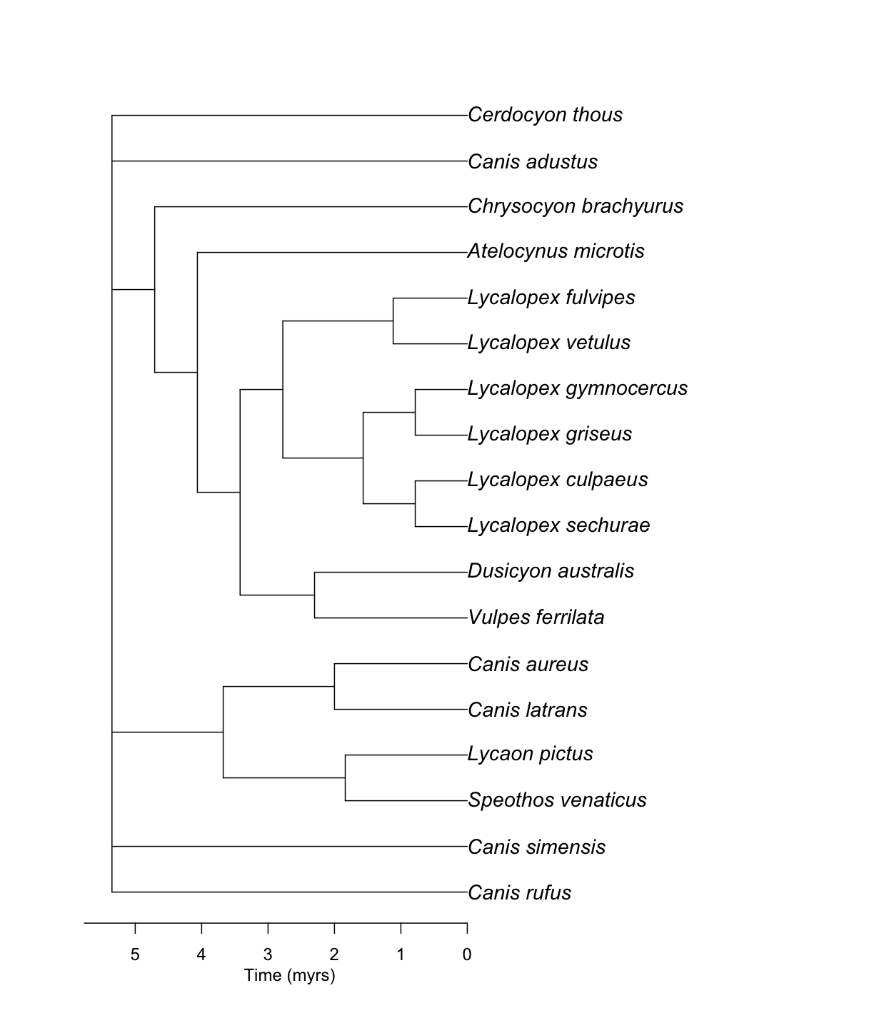
Challenge! Get the other type of summary chronogram
Hint: Explore options from the argument summary_format in the function
summarize_datelife_result()Solution
canis_phylo_sdm <- datelife::summarize_datelife_result(canis_dr, summary_format = "phylo_sdm")canis_phylo_sdmPhylogenetic tree with 18 tips and 13 internal nodes. Tip labels: Canis_rufus, Canis_simensis, Speothos_venaticus, Lycaon_pictus, Canis_latrans, Canis_aureus, ... Node labels: n1, n2, n3, n4, n5, n6, ... Unrooted; includes branch lengths.ape::plot.phylo(canis_phylo_sdm, cex = 1.2) ape::axisPhylo() graphics::mtext("Time (myrs)", side = 1, line = 2, at = max(get("last_plot.phylo",envir = .PlotPhyloEnv)$xx) * 0.5)
As you can note, the SDM sumary chronogram is slightly older than the median summary chronogram!
Finally, give it a try on the web browser of datelife, too. You can do the same things using a graphical user interface. It is fun!
Key Points
Source chronograms have a wide range of variation in age estimates.
