Physcraper Examples: the Hollies

*Ilex* fruits and leaves in the snow. Image by [Wolfgang Claussen](https://pixabay.com/es/users/WolfBlur-2503887/) at [Pixabay](https://pixabay.com/es/photos/holly-ilex-aquifolium-la-nieve-3012084/).

Ilex fruits and leaves in the snow. Image by Wolfgang Claussen at Pixabay.

I. Finding a tree to update

Using the Open Tree of Life website

Go to the Open Tree of Life website and use the “search for taxon” menu to look up for the taxon Ilex.

The screenshpt below shows the state of the genus Ilex in the Open Tree of Life synthetic tree on May 25, 2020. If you go to OpenTree’s website you can check out Ilex current state here.

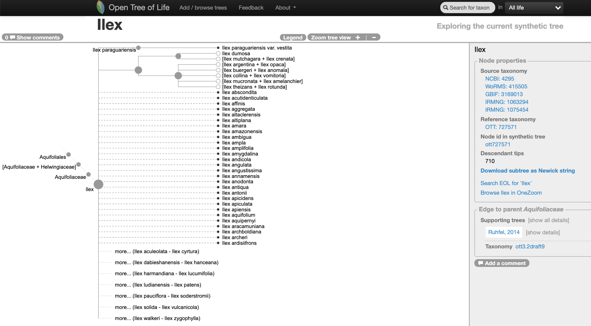
Navigating into the tree, we notice that there might be two studies associated to this portion of the Open Tree synthetic tree.

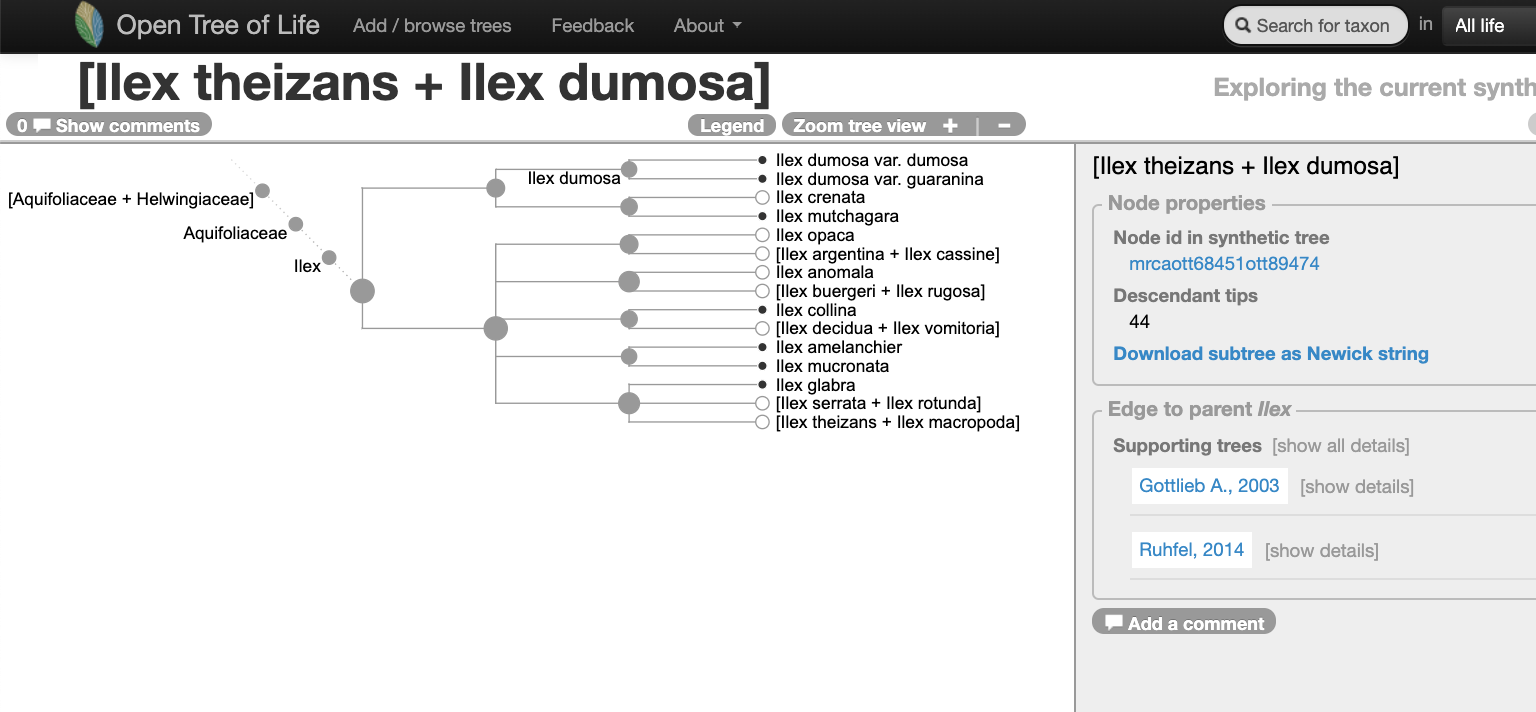
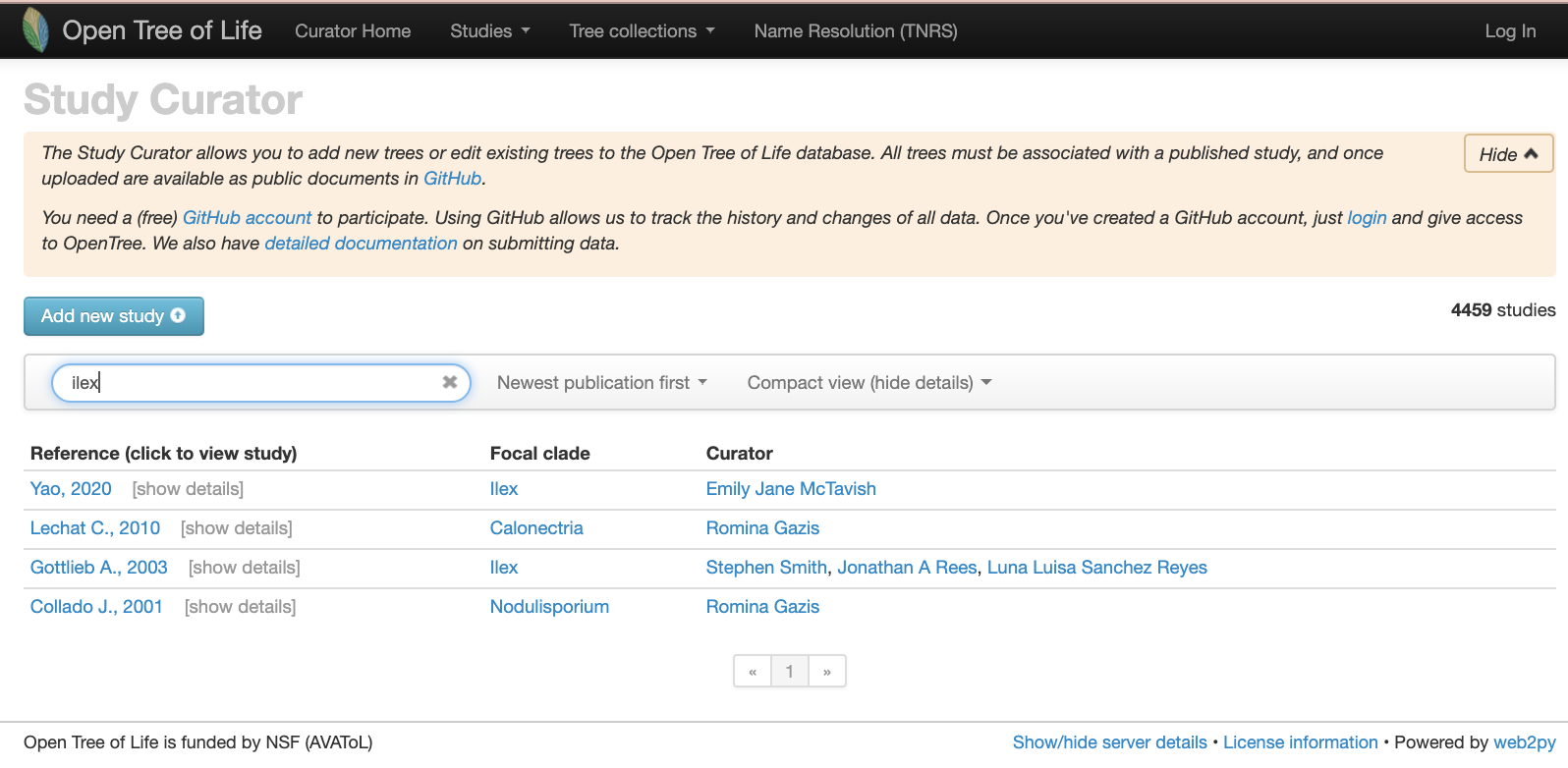
Let’s verify that on the study curator of OToL.

Studies matching the word ‘ilex’ on the curator database, at the middle of year 2020. Some of these studies are not actually about the hollies, but other taxa that have the species epithet ilex, e.g., the holly oak Quercus ilex or the rodent Apodemus ilex

Using the R package rotl

Explain what a focal clade is.

There is a handy function that will search a taxon among the focal clades reported across trees.

studies <- rotl::studies_find_studies(property="ot:focalCladeOTTTaxonName", value="Ilex")

Studies with the genus *Ilex* as focal clade.
study_ids	n_trees	tree_ids	candidate	study_year	title	study_doi
ot_1984	1	tree1		2020		http://dx.doi.org/10.1111/jse.12567
pg_2827	2	tree6576, tree6577	tree6577	2005	Molecular analyses of the genus Ilex (Aquifoliaceae) in southern South America, evidence from AFLP and ITS sequence data	http://dx.doi.org/10.3732/ajb.92.2.352

It seems like the oldest tree, tree6577 from study pg_2827, is in the Open Tree of Life synthetic tree.

Let’s get it and plot it here:

original_tree <- rotl::get_study_tree(study_id = "pg_2827", tree_id = "tree6577")
#> Warning in build_raw_phylo(ncl, missing_edge_length): missing edge lengths are
#> not allowed in phylo class. All removed.
ape::plot.phylo(ape::ladderize(original_tree), type = "phylogram", cex = 0.3, label.offset = 1, edge.width = 0.5)

Now, let’s look at some properties of the tree:

ape::Ntip(original_tree)  # gets the number of tips
#> [1] 48
ape::is.rooted(original_tree)  # check that it is rooted
#> [1] TRUE
ape::is.binary(original_tree)  # check that it is fully resolved
#> [1] FALSE
datelife::phylo_has_brlen(original_tree)  # checks that it has branch lengths
#> [1] FALSE

The tree has 48 tips, is rooted, has no branch lengths and is not fully resolved, as you probably already noted. Also, labels correspond to the labels reported on the original study here. Other labels are available to use as tip labels. For example, you can plot the tree using the unified taxonomic names, or the taxonomic ids.

Finding a tree in the Open Tree of Life phylesystem with at least one tip label belonging to the group of interest.

find_trees.py --taxon_name  "Ilex"

II. Getting the underlying alignment

From TreeBASE

Using physcraper and the arguments `-tb` and `-no_est`

physcraper_run.py -s pg_2827 -t tree6577 -tb -no_est -o data/pg_2827_tree6577

Downloading the alignment directly from a repository

The alignments are here https://treebase.org/treebase-web/search/study/matrices.html?id=1091

On a mac you can do:

wget "http://purl.org/phylo/treebase/phylows/matrix/TB2:M2478?format=nexus" -o data-raw/alignments/T1281-M2478.nex

Other repos

III. Starting a Physcraper a run

physcraper_run.py -s pg_2827 -t tree6577 -o data/pg_2827_tree6577

physcraper_run.py -s pg_2827 -t tree6577 -a data-raw/alignments/T1281-M2478.nex -as nexus -o data/ilex-remote

Using a local BLAST database

physcraper_run.py -s pg_2827 -t tree6577 -a data-raw/alignments/T1281-M2478.nex -as nexus -db local_blast_db -o data/ilex-local

IV. Reading the Physcraper results

The Pxhyscraper tag

T1281-M2478

Input files

Physcraper rewrites input files for a couple reasons: reproducibility, taxon name matching, and taxon reconciliation. It also writes the config file down if none was provided.

Run files

Files in here are also automatically written down by Physcraper.

blast runs, alignments, raxml trees, bootstrap

The trees are reconstructed using RAxML, with tip labels corresponding to Physcraper taxon ids (e.g., otu42009, otuPS1) and not taxon names (e.g., Helwingia japonica), nor taxonomic ids (e.g., ott or ncbi). Branch lengths are proportional to relative substitution rates. The RAxML tree with taxon names as tip labels is saved on the outputs_tag folder.

updated_tree_otus <- ape::read.tree(file = "../data/ilex-local/run_T1281-M2478/RAxML_bestTree.2020-06-29")
ape::plot.phylo(ape::ladderize(updated_tree_otus), type = "fan", cex = 0.25, label.offset = 0.01, edge.width = 0.5)
ape::add.scale.bar(cex = 0.3, font = 1, col = "black")
mtext("Updated tree - otu tags as labels", side = 3, line = 0)

Output files

A variety of files are automatically written down by Physcraper.

A nexson tree with all types of tip labels is saved in here. From this tree, a tree with any kind of label can be produced. By default, the updated tree with taxon names as tip labels is saved in the output_tag folder as updated_taxonname.tre.

Updated_sumtree and updated_tree_taxonname are the same tree: a consensus tree output of summtrees from DendroPy.

updated_sumtree <- ape::read.tree(file = "../data/pg_2827_tree6577/outputs_pg_2827tree6577/physcraper_pg_2827tree6577.tre")

updated_tree_taxonname <- ape::read.tree(
  file = "../data/pg_2827_tree6577/outputs_pg_2827tree6577/updated_taxonname.tre")
# ape::plot.phylo(ape::ladderize(updated_tree_taxonname), cex = 0.35)
# updated_tree_taxonname$tip.label %in% c("Helwingia_japonica_otu420083", "Helwingia_chinensis_otu420099")

# updated_raxml <- ape::read.tree(file = "../data/pg_2827_tree6577/run_pg_2827tree6577_run4/RAxML_bestTree.2020-07-31")
updated_sumtree_drop <- ape::drop.tip(updated_sumtree, c("otu420083", "otu420099"))

ape::plot.phylo(ape::ladderize(updated_tree_taxonname), type = "fan", cex = 0.25, label.offset = 0.01, edge.width = 0.5)
ape::add.scale.bar(cex = 0.3, font = 1, col = "black")
mtext("Updated tree - Taxon names as labels  ", side = 3, line = 1)

V. Visualizing the Physcraper results

#> [1] 61
#> [1] 30
#> [1] 77
#> [1] 207
#> [1] 1.000001e-06 1.000001e-06 1.000001e-06 1.000001e-06 1.000001e-06
#> [6] 1.000001e-06 1.000001e-06 2.000001e-06
#> [1] 0.96 0.95 0.95 0.93 0.76 0.76 0.93 0.86
#> [1] 6.716139e-03 1.982183e-01 1.130793e-02 1.000001e-06 8.803937e-03
#> [6] 1.000001e-06 1.138649e-02 7.447242e-03

Visualizing new tips and taxa

An easy way to visualize the new tips added into the updated tree compared to the original tree is coloring the tips and branches from those new tips with a highlighting color. We will use the function plot_branches defined in this package to do so.

The function takes as argument the paths to both the tree and the OTU info files:

# mytreefile = '../data/pg_2827_tree6577/run_pg_2827tree6577_run4/RAxML_bestTree.2020-07-31'
mytreefile = '../data/pg_2827_tree6577/outputs_pg_2827tree6577/physcraper_pg_2827tree6577.tre'
myotuinfofile = '../data/pg_2827_tree6577/outputs_pg_2827tree6577/otu_info_pg_2827tree6577.csv'

And uses phytools::plotBranchbyTrait, so it takes all arguments from ape::plot.phylo, too:

plot_branches(treefile = mytreefile, otufile = myotuinfofile, type = "phylogram", cex = 0.25, edge.width = 0.5, tip_label = "taxon", color = "goldenrod", edge_length = FALSE)
mtext(expression(Updated~italic(Ilex) ~ plain("gene tree - 4 BLAST cycles")), side= 3, line=-1, cex = 0.5)

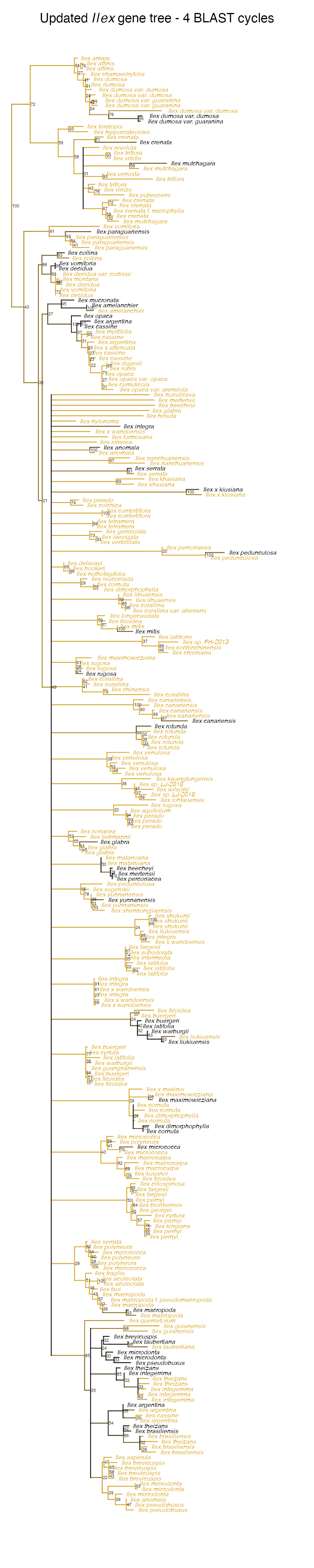
# ape::nodelabels(node=bb+ape::Ntip(updated_sumtree_drop)-1, pch =8, cex = 0.1, col = "green")  # uncomment this if you want to show tiny-tiny branches that have a large bootstrap support!

The green nodes highlight branches with a length < 0.00001 and a bootstrap support > 0.75

Let’s get the summary of new tips:

summ <- summarize(treefile = mytreefile, otufile = myotuinfofile)
#> This updated tree has 48 original tips, representing 45 unique OTT taxa.
#> And 231 new tips representing 83 new OTT taxa added to the original tree.
#> It is 0.75% resolved.
updated_sumtree_drop <- ape::ladderize(updated_sumtree_drop)
internal_edges <- updated_sumtree_drop$edge[,2] > ape::Ntip(updated_sumtree_drop)
tip_edges <- updated_sumtree_drop$edge[,2] <= ape::Ntip(updated_sumtree_drop)
boots <- as.numeric(updated_sumtree_drop$node.label)
sum(boots>0.8)
#> [1] 61
# internal edges that are very small:
sum(updated_sumtree_drop$edge.length[internal_edges]<0.00001) # 30
#> [1] 30
# tip edges that are very small:
sum(updated_sumtree_drop$edge.length[tip_edges]<0.00001) # 77
#> [1] 77
updated_sumtree_drop$Nnode
#> [1] 207
ie <- updated_sumtree_drop$edge.length[internal_edges]
ie <- c(1, ie) # adding a root edge length
sum(boots<0.75)/ape::Ntip(updated_sumtree_drop)
#> [1] 0.4873646
bb <- which(ie<0.00001 & boots>0.75)
ie[bb]
#> [1] 1.000001e-06 1.000001e-06 1.000001e-06 1.000001e-06 1.000001e-06
#> [6] 1.000001e-06 1.000001e-06 2.000001e-06
boots[bb]
#> [1] 0.96 0.95 0.95 0.93 0.76 0.76 0.93 0.86
updated_sumtree_drop$edge.length[bb+ape::Ntip(updated_sumtree_drop)]
#> [1] 6.716139e-03 1.982183e-01 1.130793e-02 1.000001e-06 8.803937e-03
#> [6] 1.000001e-06 1.138649e-02 7.447242e-03
ss <- sapply(bb+ape::Ntip(updated_sumtree_drop)-1, function(x)
              phytools::getDescendants(tree=updated_sumtree_drop, node=x))

hist(updated_sumtree_drop$edge.length, breaks=1400, col = "skyblue3",
     border = "skyblue3", xlab= "Branch Length (substitution rate)",
     main = "Updated Gottlieb2005 tree \n branch length frequency distribution")

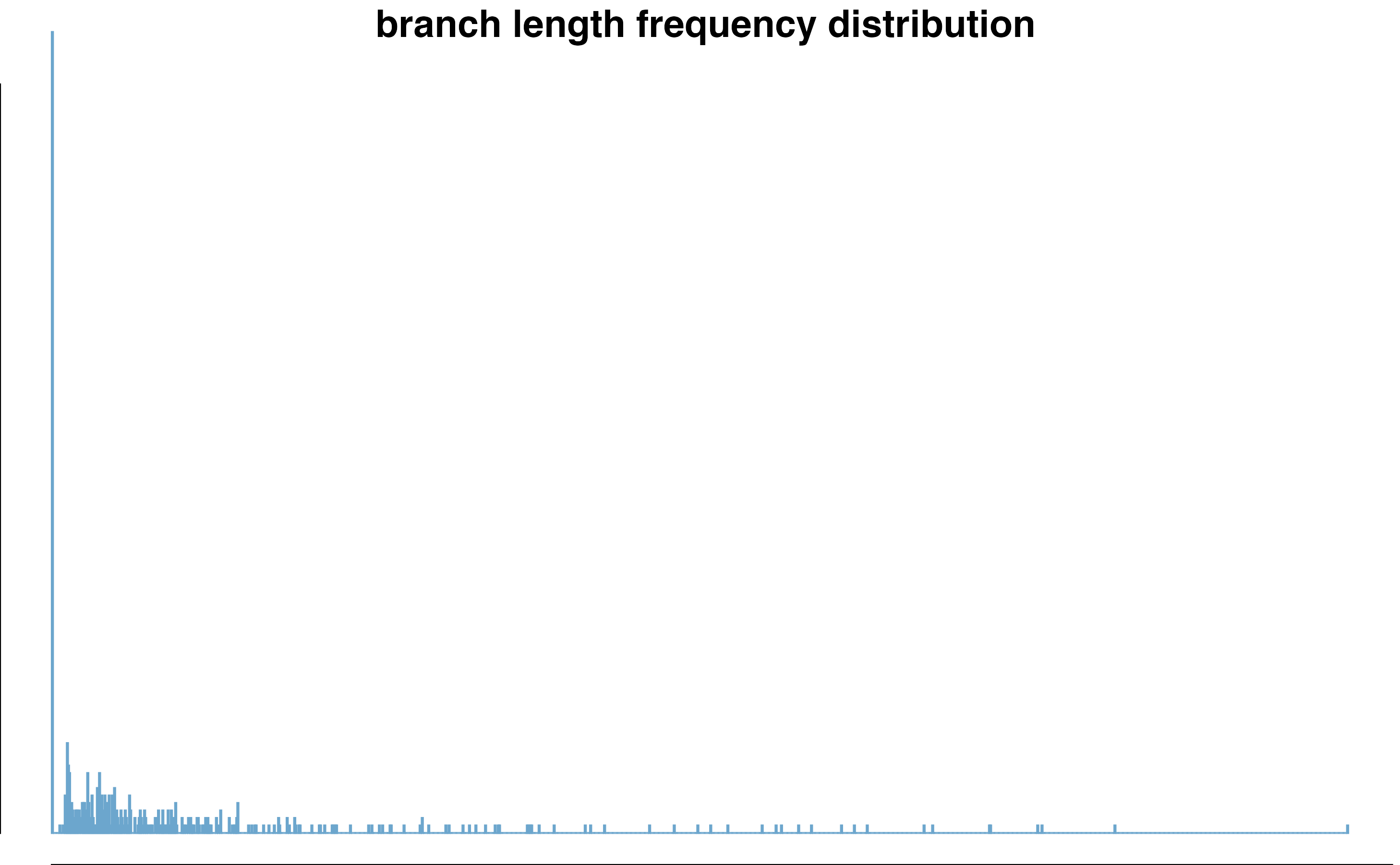
This branch length distribution excludes the outgroup branches, it contains branches from the ingroup only.

The updated tree is 75% resolved, with 249 branches that are <0.01 and 107 are < 0.00001, effectively negligible. The longest branch is 0.2416085 and the smallest branch is 1.000000510^{-6}

V. Comparing the Physcraper results

Visualizing changes in phylogenetic relationships

How do the phylogenetic relationships from the updated tree compare to those from the original tree and other Ilex trees?

We will use the conflict tool of the OpenTree to visualize this.

The next figure shows in green the nodes resolved by the Gottlieb2005 tree and in blue the nodes that align with taxonomy: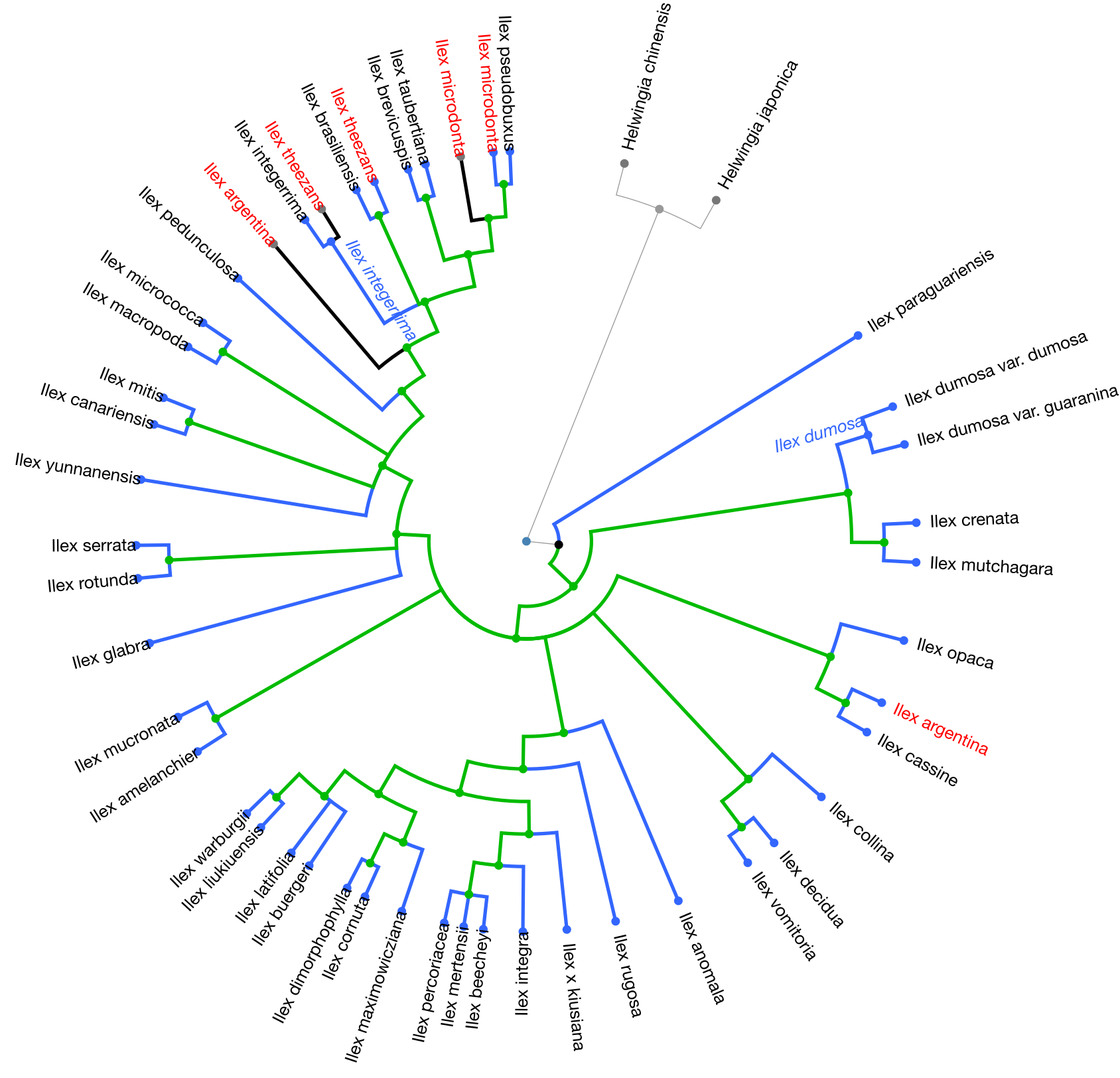

The following figure shows results from the conflict analysis in the updated Ilex tree. The blue nodes either align with phylogenetic relationships from the Gottlieb2005 tree or with taxonomy; the green nodes (approximately 20) resolve phylogenetic relationships that were not solved by Gottlieb2005; and the orange nodes conflict either with phylogenetic relationships shown in Gottlieb2005 or with taxonomy.

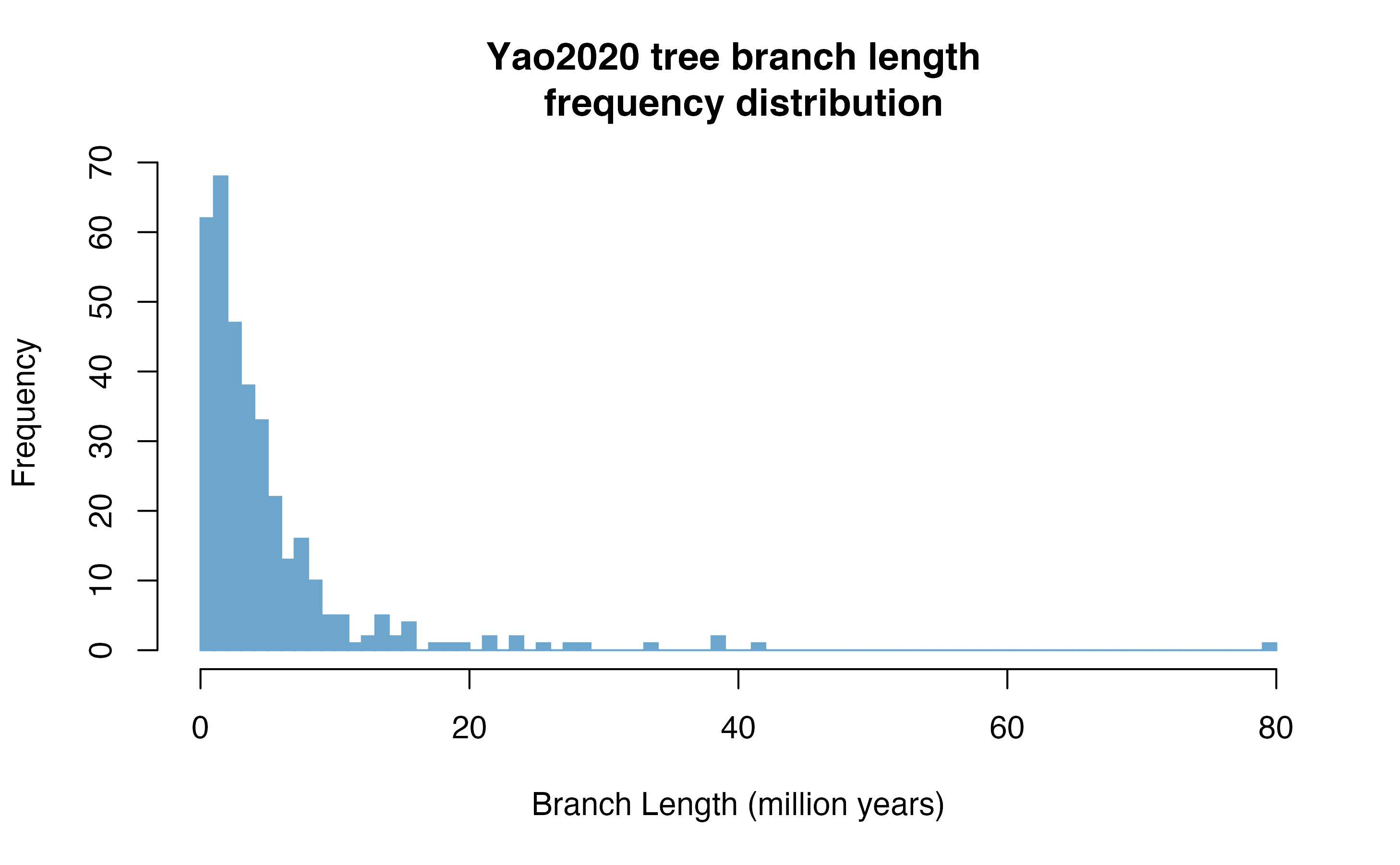
Let’s get the Yao2020 tree:

yao2020 <- rotl::get_study_tree(study_id = "ot_1984", tree_id = "tree1")

hist(yao2020$edge.length, col = "skyblue3", breaks = round(max(yao2020$edge.length)),
     border = "skyblue3", xlab= "Branch Length (million years)",
     main = "Yao2020 tree branch length \n frequency distribution")

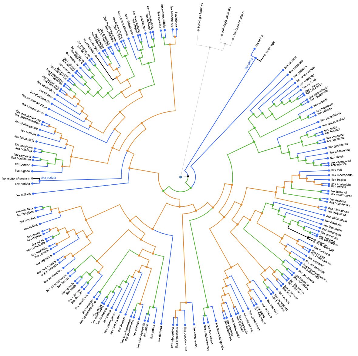
Now we can compare the taxa in the updated Gottlieb2005 and in Yao2020:

comp <- compare(treefile = mytreefile, otufile = myotuinfofile, tree = yao2020)
#> The updated tree (from treefile) and the tree to compare (from tree)
#>   contribute jointly with 151 distinct taxa that are in not in the original tree.
#>  From this, 65 taxa are present in both trees.
#> The updated tree contributes 18 distinct taxa that are neither in original tree
#>   nor in tree to compare.
#> The tree to compare has 133 new tips and contributes 133 distinct taxa 
#>  from which 68 are neither in original tree nor in the updated tree.
#> The tree to compare has 42 taxa that are in original tree.
#> And 133 tips different from original, representing 68 new OTT taxa added to the original tree.
#> It is 0.99% resolved.

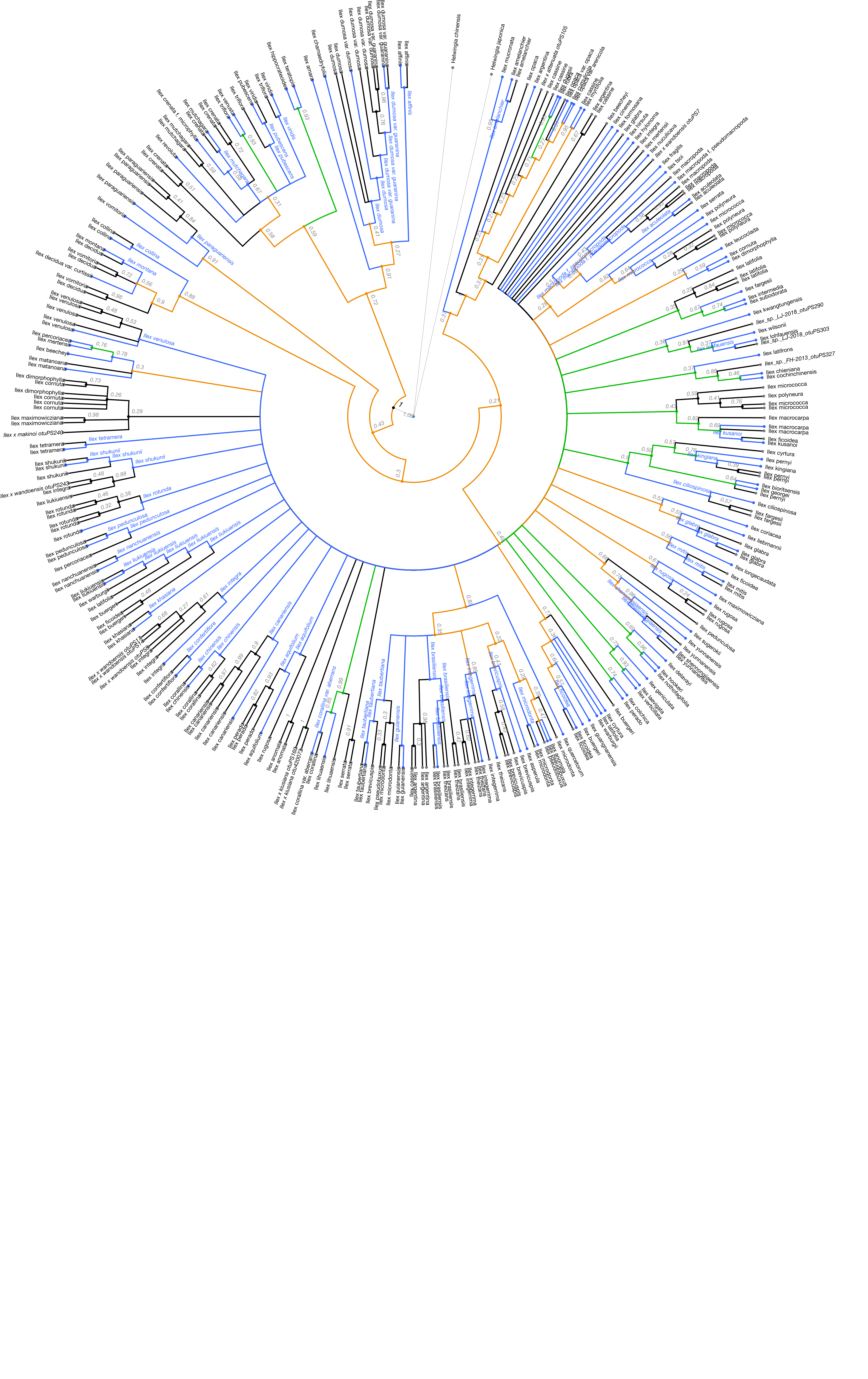
The following figure shows results from the conflict analysis on the Yao2020 tree. Again, the blue nodes align either with Gottlieb2005 or with taxonomy, the green nodes (approximately 80) resolve phylogenetic relationships that were not solved by Gottlieb2005, and the orange nodes conflict either with phylogenetic relationships from Gottlieb2005 or with taxonomy.

With Python:

from opentree import OT
import physcraper

gottleib_updated = physcraper.treetaxon.generate_TreeTax_from_run("../physcraperex/data/ilex-local/")
gottleib_updated.write_labelled(path = "gott_taxonlab.tre",label = '^ot:ottTaxonName', norepeats=False)

The following generates a tree with tip labels with spaces instead of underscores.

yao = OT.get_tree(study_id="ot_1984", tree_id="tree1",tree_format = "newick", label_format='ot:ottTaxonName')
fi = open("yao.tre", "w")
fi.write(yao.response_dict['content'].decode())
fi.close()

Use the tree comparison script:

tree_comparison.py -t1 gott_taxonlab.tre -t2 yao.tre -og otu468906 otu1030991 -otu data/pg_2827_tree6577/outputs_pg_2827tree6577/otu_info_pg_2827tree6577.csv -o ilex_comparison

Acknowledgments

Research was supported by the grant “Sustaining the Open Tree of Life”, National Science Foundation ABI No. 1759838, and ABI No. 1759846.

Computer time was provided by the Multi-Environment Research Computer for Exploration and Discovery (MERCED) cluster from the University of California, Merced (UCM), supported by the NSF Grant No. ACI-1429783.