#> [1] "/Users/luna/pj_physcraper/physcraperex/vignettes"

Cocoa plant fruits

I. Finding a tree to update

With the Open Tree of Life website

Go to the Open Tree of Life website and use the “search for taxon” menu to look up the taxon Malvaceae.

This is how the genus Malvaceae is represented on the Open Tree of Life synthetic tree at the middle of year 2020:

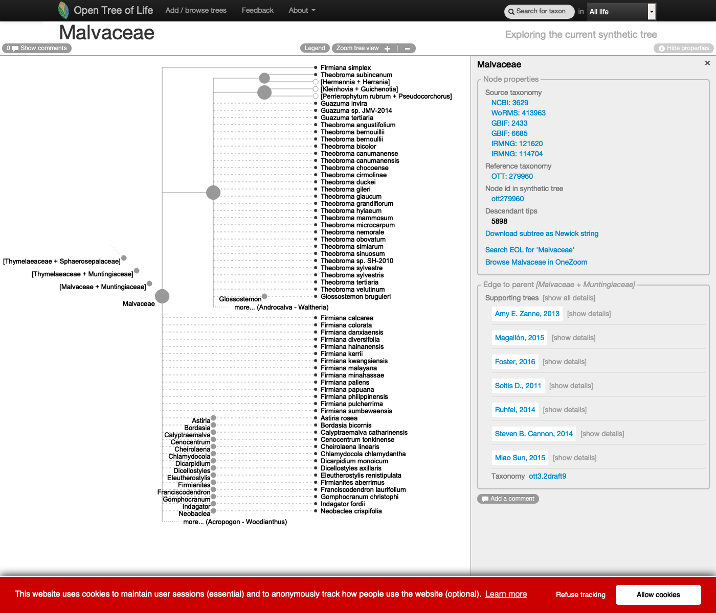
See this live on the website at https://tree.opentreeoflife.org/opentree/argus/ottol@279960/Malvaceae

Let’s go to the study curator of OToL and look up for uploaded studies for the Malvaceae

Studies matching the word ‘malvaceae’ on the curator database, at the middle of year 2020. Some of these studies are not actually about the Malvaceae, but other taxa that have the keyword malvaceae.

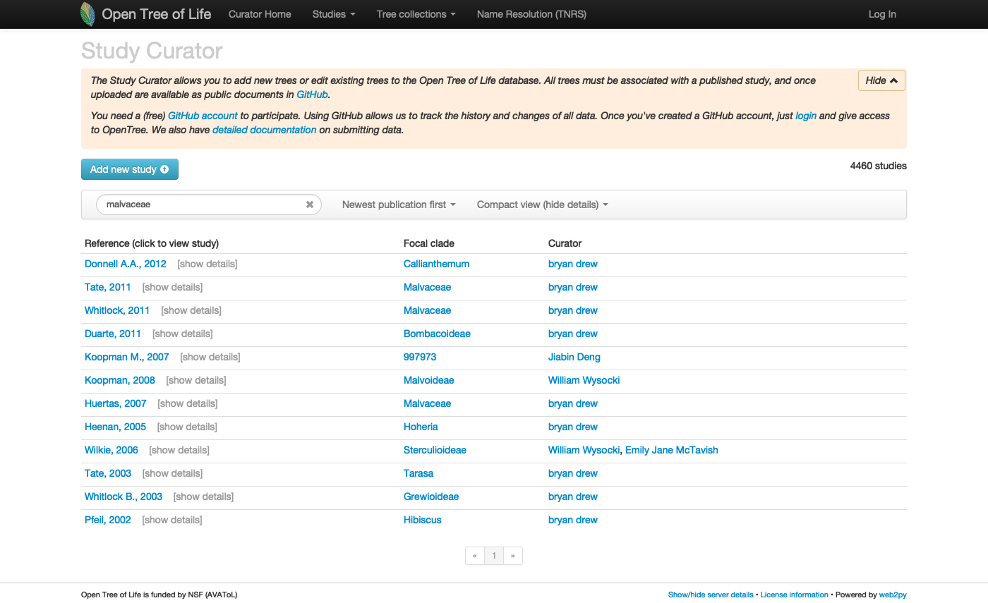
See this live on the curator app at https://tree.opentreeoflife.org/curator/?match=malvaceae

Finding a tree to update using the R package rotl

Explain what a focal clade is.

There is a handy function that will search a taxon among the focal clades reported across trees.

studies <- rotl::studies_find_studies(property="ot:focalCladeOTTTaxonName", value="Malvaceae")

Studies with the genus *Malvaceae* as focal clade.
study_ids	n_trees	tree_ids	study_year	study_doi
pg_628	3	tree1029, tree1030, tree5358	2011
pg_629	1	tree1031	2010	http://dx.doi.org/10.1600/036364411X553216
pg_1855	4	tree3745, tree3746, tree3747, tree3748	2007	http://dx.doi.org/10.1600/036364407780360157

None of these trees are in the synthetic tree. Still, the family does not appear as a politomy and has phylogenetic information in the Open Tree of Life synthetic tree. Where is this information coming from?

It is probably coming from studies with focal clades that might be either above or below the particular clade we are interested in!

You can get supporting trees with the Open Tree of Life API, and you can currently do it now using a hidden rotl function:

res <- rotl:::.tol_subtree(ott_id=279960)
# studies <- rotl:::studies_from_otl(res) # not supported anymore as of April 2021
# studies

Updating study `pg_55`

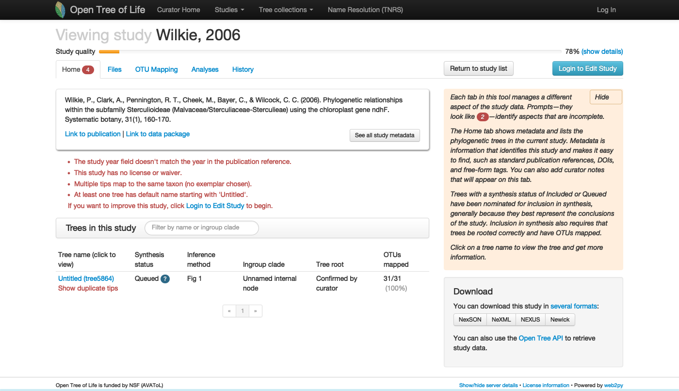
See this live on the curator app at https://tree.opentreeoflife.org/curator/study/view/pg_55

pg_55_meta = rotl::get_study_meta(study_id = "pg_55")
ls(pg_55_meta$nexml)
pg_55_meta$nexml$treesById
unlist(pg_55_meta$nexml$treesById)[1]
# rotl::taxonomy_taxon_info(pg_55_meta$nexml$"^ot:focalClade")
#>  [1] "@generator"                    "@id"                          
#>  [3] "@nexml2json"                   "@nexmljson"                   
#>  [5] "@version"                      "@xmlns"                       
#>  [7] "^ot:agents"                    "^ot:annotationEvents"         
#>  [9] "^ot:candidateTreeForSynthesis" "^ot:comment"                  
#> [11] "^ot:curatorName"               "^ot:dataDeposit"              
#> [13] "^ot:focalClade"                "^ot:focalCladeOTTTaxonName"   
#> [15] "^ot:otusElementOrder"          "^ot:studyId"                  
#> [17] "^ot:studyPublication"          "^ot:studyPublicationReference"
#> [19] "^ot:studyYear"                 "^ot:tag"                      
#> [21] "^ot:treesElementOrder"         "otusById"                     
#> [23] "treesById"                    
#> $trees55
#> $trees55$treeById
#> $trees55$treeById$tree5864
#> NULL
#> 
#> 
#> $trees55$`^ot:treeElementOrder`
#> $trees55$`^ot:treeElementOrder`[[1]]
#> [1] "tree5864"
#> 
#> 
#> $trees55$`@otus`
#> [1] "otus55"
#> 
#> 
#> trees55.^ot:treeElementOrder 
#>                   "tree5864"

The focal clade of study is Sterculioideae. Is this taxon in the synthetic tree? FALSE

Let’s get the original tree and plot it here:

original_tree <- rotl::get_study_tree(study_id = "pg_55", tree_id = "tree5864")
ape::plot.phylo(ape::ladderize(original_tree), type = "phylogram", cex = 0.3, label.offset = 1, edge.width = 0.5)
mtext("Original tree - original labels", side = 3, cex = 0.6)

Now, let’s look at some properties of the tree:

ape::Ntip(original_tree)  # gets the number of tips
#> [1] 31
ape::is.rooted(original_tree)  # check that it is rooted
#> [1] FALSE
ape::is.binary(original_tree)  # check that it is fully resolved
#> [1] FALSE
datelife::phylo_has_brlen(original_tree)  # checks that it has branch lengths
#> [1] FALSE

The tree has 31 tips, is rooted, has no branch lengths and is not fully resolved, as you probably already noticed. Also, labels correspond to the labels reported on the original study here. Other labels are available to use as tip labels. For example, you can plot the tree using other labels, like the unified taxonomic names, or the taxonomic ids.

II. Getting the underlying alignment

Using physcraper and the arguments `-tb` and `-no_est`

This will download the alignment directly from TreeBASE:

physcraper_run.py -s pg_55 -t tree5864 -tb -no_est -o data/pg_55

The alignment will be saved as pg_55tree5864.aln and physcraper_pg_55tree5864.fas in the inputs folder.

Downloading the alignment directly from a repository

We know that the alignments are in the TreeBASE repo at https://treebase.org/treebase-web/search/study/matrices.html?id=1361

Let’s save them to a file named TB2:Tr240.nex in the data-raw/alignments folder:

wget -O data-raw/alignments/TB2:Tr240.nex "http://purl.org/phylo/treebase/phylows/tree/TB2:Tr240?format=nexus"

III. Starting a physcraper run

We ran this example using the command:

physcraper_run.py -s pg_55 -t tree5864 -a data-raw/alignments/TB2:Tr240.nex -as nexus -o data/pg_55

IV. Reading the physcraper results

The physcraper tag

pg_55tree5864_ndhf

Input files

Physcraper rewrites input files for a couple reasons: reproducibility, taxon name matching, and taxon reconciliation. It writes the config file down if none was provided. Everything is written into the inputs_tag folder.

Run files

Files in here are also automatically written down by physcraper.

blast runs, alignments, raxml trees, bootstrap

The trees are reconstructed using RAxML, with tip labels corresponding to local ids (e.g., otu42009, otuPS1) and not taxon names (e.g., Ceiba), nor taxonomic ids (e.g., ott or ncbi). Branch lengths are proportional to relative substitution rates. The RAxML tree with taxon names as tip labels is saved on the outputs_tag folder.

updated_tree_otus <- ape::read.tree(file = "../data/pg_55/run_pg_55tree5864_ndhf/RAxML_bestTree.2020-06-09")
ape::plot.phylo(ape::ladderize(updated_tree_otus), type = "phylogram", cex = 0.25, label.offset = 0.001, edge.width = 0.5)
ape::add.scale.bar(cex = 0.3, font = 1, col = "black")
mtext("Updated tree - otu tags as labels", side = 3)

Output files

A number of files is automatically written down by physcraper.

A nexson tree with all types of tip labels is saved in here. From this tree, a tree with any kind of label can be produced. By default, the updtaed tree with taxon names as tip labels is saved in the output_tag folder as updated_taxonname.tre.

updated_tree_taxonname <- ape::read.tree(
  file = "../data/pg_55/outputs_pg_55tree5864_ndhf/updated_taxonname.tre")
updated_tree_taxonname$tip.label.original <- updated_tree_taxonname$tip.label

ape::plot.phylo(ape::ladderize(updated_tree_taxonname), type = "phylogram", cex = 0.2, label.offset = 0.001, edge.width = 0.5)
ape::add.scale.bar(cex = 0.3, font = 1, col = "black")
mtext("Updated tree - Taxon names as labels", side = 3)

IV. Analyzing the physcraper results

Compare the original tree with the pruned updated tree

original_tree_otus <- ape::read.tree(file = "../data/pg_55/inputs_pg_55tree5864_ndhf/physcraper_pg_55tree5864_ndhf.tre")
updated_tree_otus_pruned <- ape::read.tree(
  file = "../data/pg_55/pruned_updated.tre"
)
# This tree only has 31 tips because it is the pruned updated tree.

Lets get indices from the new tips added to the updated tree and see which taxa they correspond to:

new_tips <- grep("_otuPS[0-9]*", updated_tree_taxonname$tip.label.original)
updated_tree_taxonname$tip.label.original[new_tips]
#>  [1] "Fremontodendron_californicum_otuPS13"       
#>  [2] "Quararibea_costaricensis_otuPS38"           
#>  [3] "Matisia_cordata_otuPS39"                    
#>  [4] "Hibiscus_bojerianus_otuPS45"                
#>  [5] "Macrostelia_laurina_otuPS29"                
#>  [6] "Talipariti_tiliaceum_var._tiliaceum_otuPS48"
#>  [7] "Talipariti_hamabo_otuPS47"                  
#>  [8] "Papuodendron_lepidotum_otuPS46"             
#>  [9] "Cephalohibiscus_peekelii_otuPS34"           
#> [10] "Kokia_kauaiensis_otuPS32"                   
#> [11] "Kokia_drynarioides_otuPS31"                 
#> [12] "Kokia_cookei_otuPS30"                       
#> [13] "Ochroma_pyramidale_otuPS40"                 
#> [14] "Catostemma_fragrans_otuPS37"                
#> [15] "Scleronema_micranthum_otuPS44"              
#> [16] "Cavanillesia_platanifolia_otuPS50"          
#> [17] "Spirotheca_rosea_otuPS42"                   
#> [18] "Bombax_buonopozense_otuPS49"                
#> [19] "Ceiba_acuminata_otuPS36"                    
#> [20] "Ceiba_crispiflora_otuPS41"                  
#> [21] "Pachira_aquatica_otuPS35"                   
#> [22] "Septotheca_tessmannii_otuPS11"              
#> [23] "Triplochiton_zambesiacus_otuPS43"           
#> [24] "Sterculia_tragacantha_otuPS28"

There are 24 new tips in the updated tree.

Now plot the trees face to face.

We can first prune the updated tree of the new tips, so it is a straight forward comparison:

cotree <-  phytools::cophylo(original_tree_otus, updated_tree_otus_pruned, rotate.multi =TRUE)

Rotating nodes to optimize matching… Done.

phytools::plot.cophylo(x = cotree, fsize = 0.5, lwd = 0.5, mar=c(.1,.2,2,.3), ylim=c(-.1,1), scale.bar=c(0, .05))
title("Original tr.   Pruned updated tr.", cex = 0.1)

But it is more interesting to plot it with all the new tips, so we see exactly where the new things are:

original_tree_taxonname <- ape::read.tree(file = "../data/pg_55/inputs_pg_55tree5864_ndhf/taxonname.tre")
cotree2 <-  phytools::cophylo(
  original_tree_taxonname,
  updated_tree_taxonname,
  rotate.multi =TRUE)

Rotating nodes to optimize matching… Done.

phytools::plot.cophylo(
  x = cotree2,
  fsize = 0.3,
  lwd = 0.4,
  mar=c(.1,.1,2,.5),
  ylim=c(-.1,1),
  scale.bar=c(0, .05),
  # link.type="curved",
  link.lwd=3,
  link.lty="solid",
  link.col=phytools::make.transparent("#8B008B",0.5))
title("Original tree      Updated tree", cex = 0.1)

We can also plot the updated tree against the synthetic subtree of Malvaceae, to visualize how it updates our current knowledge of the phylogenetic relationships within the family:

tolsubtree <- rotl::tol_subtree(ott_id = 279960)

ape::Ntip(tolsubtree)
#> [1] 5898

head(tolsubtree$tip.label)
#> [1] "Perrierophytum_rubrum_ott3190"       
#> [2] "Perrierophytum_humbertii_ott3195"    
#> [3] "Kosteletzkya_reflexiflora_ott524595" 
#> [4] "Kosteletzkya_velutina_ott524593"     
#> [5] "Perrierophytum_glomeratum_ott6118239"
#> [6] "Perrierophytum_hispidum_ott6118240"
head(updated_tree_taxonname$tip.label)
#> [1] "Fremontodendron_californicum_otuPS13"       
#> [2] "Quararibea_costaricensis_otuPS38"           
#> [3] "Matisia_cordata_otuPS39"                    
#> [4] "Hibiscus_bojerianus_otuPS45"                
#> [5] "Macrostelia_laurina_otuPS29"                
#> [6] "Talipariti_tiliaceum_var._tiliaceum_otuPS48"

ape::Ntip tells us that there are almost 6k taxa in the Malvaceae OpenTree synthetic tree.

Tip labels in both trees have taxon identifier tags that will make name matching impossible. Lets remove them:

updated_tree_taxonname$tip.label <- gsub("_otuPS[0-9]*", "", updated_tree_taxonname$tip.label.original)
updated_tree_taxonname$tip.label <- gsub("_otu[0-9]*", "", updated_tree_taxonname$tip.label)

tolsubtree$tip.label.original <- tolsubtree$tip.label
tolsubtree$tip.label <- gsub("_ott[0-9]*", "", tolsubtree$tip.label)

Eliminate ott and otu tags before comparison, otherwise nothing matches

# cotree3 <-  phytools::cophylo(tolsubtree, updated_tree_taxonname, rotate.multi =TRUE)
# phytools::plot.cophylo(x = cotree3, fsize = 0.2, lwd = 0.5, mar=c(.1,.1,2,.3), ylim=c(-.1,1), scale.bar=c(0, .05))
# title("Tol subtree      Updated tree", cex = 0.1)

The whole Malvaceae tree might be too large for a cotree plot. Lets try something else.

First, get indices of new tips from updated tree present in the Malvaceae synthetic tree:

all_updated_tree_in_tol <- match(updated_tree_taxonname$tip.label, tolsubtree$tip.label)
new_tips_in_tol <- match(updated_tree_taxonname$tip.label[new_tips], tolsubtree$tip.label)
# one tip seems to be absent frm the Malvaceae subtree
updated_tree_taxonname$tip.label[47]
#> [1] "Firmiana_platanifolia"
# going to OpenTree it looks like it atually corresponds to Firmiana simplex, not sure why it was not standardized, probably bc it was in NCBI
# I'm changing it by hand:
updated_tree_taxonname$tip.label[47] <- "Firmiana_simplex"
# And running match again
new_in_tol <- match(updated_tree_taxonname$tip.label, tolsubtree$tip.label)

Then, use the `phytools package to create a data object that will contain info from our tolsubtree tips and edges:

tolsubtree <- ape::ladderize(tolsubtree)

tip_colors <- rep("gray", ape::Ntip(tolsubtree))
tip_colors[all_updated_tree_in_tol] <- "black"
tip_colors[new_tips_in_tol] <- "red"

tip_values <- rep(0, ape::Ntip(tolsubtree))
tip_values[tip_colors == "black"] <- 1
tip_values[tip_colors == "red"] <- 100
names(tip_values) <- tolsubtree$tip.label
head(tip_values)
#>     Perrierophytum_rubrum  Perrierophytum_humbertii Kosteletzkya_reflexiflora 
#>                         0                         0                         0 
#>     Kosteletzkya_velutina Perrierophytum_glomeratum   Perrierophytum_hispidum 
#>                         0                         0                         0
all_values <- sum_tips(tolsubtree, tip_values)

all_cols <- rep("gray", length(all_values))
all_values[all_values >= 100]
#>   [1]  100  100  100  100  100  100  100  100  100  100  100  100  100  100  100
#>  [16]  100  100  100  100  100  100  100  100  100 2422 2413 2413 2413 2413 2413
#>  [31] 2413 2313 2213 1213 1013  900  700  700  700  400  100  100  300  300  200
#>  [46]  200  200  100  100  100  100  100  100  100  100  100  100  300  300  300
#>  [61]  300  300  200  200  100  113  109  109  105  101  100  100  100 1000  800
#>  [76]  800  300  300  200  100  100  100  500  100  100  400  200  200  100  100
#>  [91]  200  200  100  100  100  200  100  100  100  100  100  100  100  100
all_values[all_values >= 1]
#>   [1]  100  100  100  100  100  100  100  100  100    1  100    1    1    1    1
#>  [16]    1    1    1    1    1    1    1    1  100  100  100  100  100  100  100
#>  [31]  100  100  100  100  100  100  100    1    1    1    1    1    1    1    1
#>  [46]    1 2422 2413 2413 2413 2413 2413 2413 2313 2213 1213 1013  900  700  700
#>  [61]  700  400  100  100  300  300  200  200  200  100  100  100  100  100  100
#>  [76]  100  100  100  100  300  300  300  300  300  200  200  100  113  109  109
#>  [91]  105  101    1  100  100    4    4    1    4    3    2    2    1    1  100
#> [106] 1000  800  800  300  300  200  100  100  100  500  100  100  400  200  200
#> [121]  100  100  200  200  100  100  100  200  100  100  100  100  100  100  100
#> [136]  100    1    2    2    1    1

all_cols[all_values >= 1] <- "black"
all_cols[all_values >= 100] <- "red"
edge_colors <- all_cols[tolsubtree$edge[,2]]
length(edge_colors) == nrow(tolsubtree$edge)
#> [1] TRUE
# tip_cols <- all_cols[seq(ape::Ntip(tolsubtree))]

namess <- rep("Synth tips", length(edge_colors))
namess[which(edge_colors == "black")] <- "Original tips"
namess[which(edge_colors == "red")] <- "Updated tips"

tolsubtree$maps <- as.list(rep(1, length(edge_colors)))
for (i in seq(length(edge_colors))){
  names(tolsubtree$maps[[i]]) <- namess[i]
}
# fam_tree_brlen3$maps[1]
# str(fam_tree_brlen3$maps)
cols <- setNames(c("red","black", "gray"), c("Updated tips", "Original tips", "Synth tips"))
tolsubtree_wbl <- ape::compute.brlen(tolsubtree)
tolsubtree_wbl$maps <- tolsubtree$maps

par(fg="transparent")
phytools::plotSimmap(tolsubtree_wbl,type="fan",part=0.95, ftype="i", colors = cols, lwd = 0.1, fsize = 0.05) #lwd = 0.5, fsize=0.1
lastPP<-get("last_plot.phylo",env=.PlotPhyloEnv)
par(fg="black")
phytools::add.simmap.legend(colors=cols,vertical=FALSE,x=-0.9, y=-1.2,prompt=FALSE, fsize = 0.5)
tt<-gsub("_"," ",tolsubtree_wbl$tip.label)
#tt[tip_colors == "gray"] <- ""
text(lastPP$xx[1:length(tt)],lastPP$yy[1:length(tt)],
  tt,cex=0.2,col=tip_colors,pos=4,offset=0.1,font=3)

References

Trick for the cophylo titles and margins from https://cran.r-project.org/web/packages/phangorn/vignettes/IntertwiningTreesAndNetworks.html

Trick for colord tip labels: http://blog.phytools.org/2013/09/coloring-tip-labels-by-character-state.html

Physcraper Examples: the Malvaceae